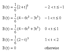
B Spline functions
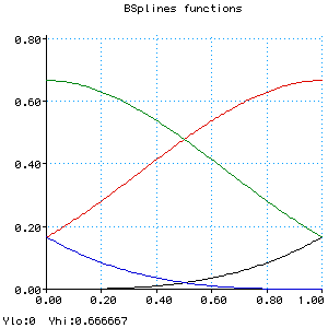
Bi(u) = (u^3)/6Bi-1(u) = (-3*(u^3) + 3*(u^2) + 3*u +1)/6 Bi-2(u) = (3*(u^3) - 6*(u^2) +4)/6 Bi-3(u) = (1 - u)^3/6 |
 |
Bi(u) = (u^3)/6Bi-1(u) = (-3*((u-1)^3) + 3*((u-1)^2) + 3*(u-1) +1)/6 Bi-2(u) = (3*((u-2)^3) - 6*((u-2)^2) +4)/6 Bi-3(u) = (1 - (u-3))^3/6 |
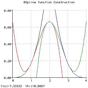 |
Bi(u) = (u^3)/6
Bi-1(u) = (-3*((u-1)^3) + 3*((u-1)^2) + 3*(u-1) +1)/6
Bi-2(u) = (3*((u-2)^3) - 6*((u-2)^2) +4)/6
Bi-3(u) = (1 - (u-3))^3/6

B(u) = Bi(u) when 0 <= u < 1,
       Bi-1(u) when 1 <= u < 2,
       Bi-2(u) when 2 <= u < 3,
       Bi-3(u) when 3 <= u < 4
|
 |
Bi(u) = (u^3)/6
Bi1(u) = (-3*((u-1)^3) + 3*((u-1)^2) + 3*(u-1) +1)/6
Bi2(u) = (3*((u-2)^3) - 6*((u-2)^2) +4)/6
Bi3(u) = (1 - (u-3))^3/6
B(u) = Bi(u) when 0 <= u < 1,
Bi1(u) when 1 <= u < 2,
Bi2(u) when 2 <= u < 3,
Bi3(u) when 3 <= u < 4
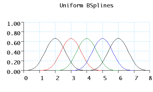
B1(u) = B(u-1)
B2(u) = B(u-2)
B3(u) = B(u-3)
B4(u) = B(u-4)
|
 |
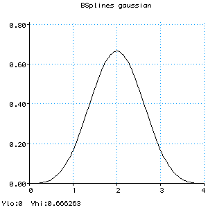
To calculate the curve at any parameter t we place a gaussian
curve over the parameter space. This curve is actually an approximation of a
gaussian; it does not extend to infinity at each end, just to +/- 2 by using
the following equations:
The Approximate Gaussian Curve
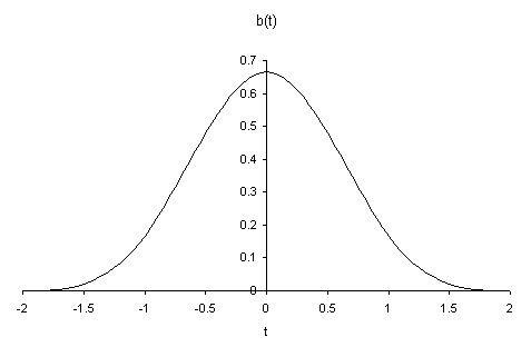
This curve peaks at a value of 2/3, and at +/- 1 its value is 1/6. When this
curve is placed over the array of control points, it gives the weighting of
each point. As the curve is drawn, each point will in turn become the heaviest
weighted, therefore we gain more local control.