eScience Lectures Notes : Surface and volume Modeling
Surface Modeling
Intro
Implicit Functions
Polygon Surfaces
Polygon Tables
Example: Plane Equations
Polygon Meshes
From Curves to Surfaces
Parametric Cubic Curves and Bicubic Patches Using Spline
Beziér Patches
Example: The Utah Teapot
Subdivision of Beziér Surfaces
Deforming a Patch
Patch Representation vs. Polygon Mesh
Constructive Solid-Geometry Methods (CSG)
Sweep Representations
A CSG Tree Representation
Implementation with ray casting
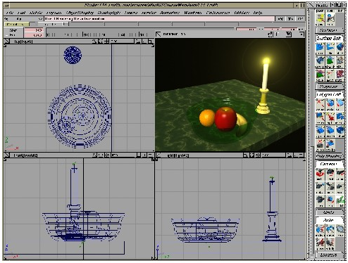
Example Modeling Package: Alias Studio
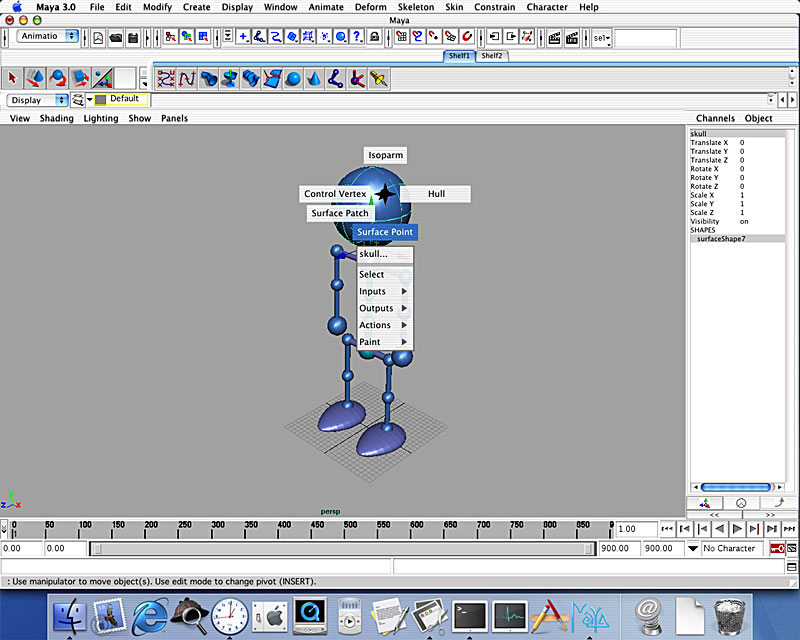
Example Modeling Package: Maya
Volume Modeling
Marching Cubes Algorithm
Marching Cube Cases
Extracted Polygonal Mesh
Metaballs
Procedural Techniques: Fractals
Procedural Modeling... L-System
Physically Based Modelling Methods
Spring Networks
Particle Systems
Surface Modeling
Types:
Polygon surfaces
Curved surfaces
Volumes
Generating models:
Interactive
Procedural
Implicit Functions vs Parametric
Implicit
The family of quadric surfaces
Or : "here is a sphere" : (O,r)
Parametric
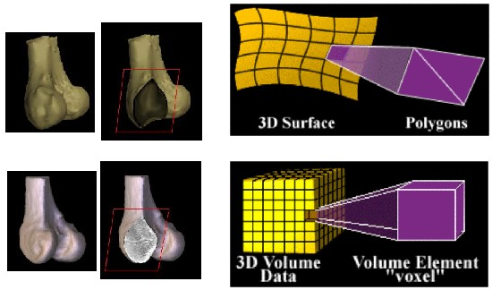
![]()
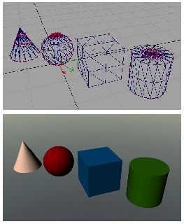
Polygon Surfaces
Set of surface polygons that enclose an object interior
 |
|
  |
How do we represent these polygons ... ?
Polygon Tables
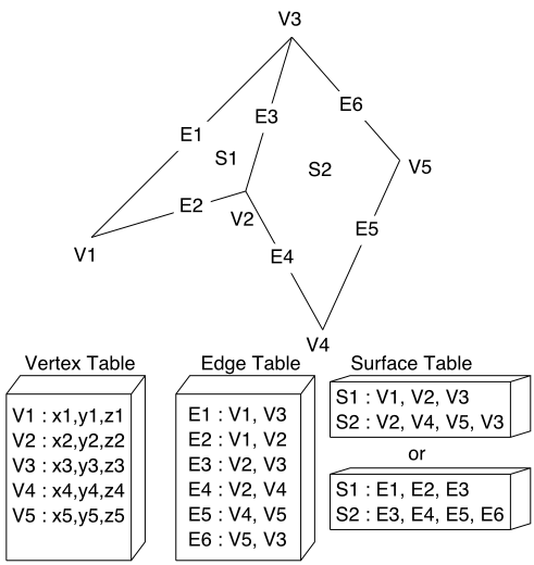
We specify a polygon surface with a set of vertex coordinates and associated attribute parameters
|
Objects : set of vertices and associated attributes Geometry : stored as three tables : vertex table, edge table, polygon table Edge table ? Tables also allow to store additional information |
 |
|---|
- We specify objects as a set of vertices and associated attributes.
This information can be stored in tables, of which there are two types: geometric tables and attribute tables. - The geometry can be stored as three tables: a vertex table, an edge table, and a polygon table. Each entry in the vertex table is a list of coordinates defining that point. Each entry in the edge table consists of a pointer to each endpoint of that edge. And the entries in the polygon table define a polygon by providing pointers to the edges that make up the polygon.
- We can eliminate the edge table by letting the polygon table reference the vertices directly, but we can run into problems, such as drawing some edges twice, because we don't realize that we have visited the same set of points before, in a different polygon. We could go even further and eliminate the vertex table by listing all the coordinates explicitly in the polygon table, but this wastes space because the same points appear in the polygon table several times.
- Using all three tables also allows for certain kinds of error checking. We can confirm that each polygon is closed, that each point in the vertex table is used in the edge table and that each edge is used in the polygon table.
- Tables also allow us to store additional information. Each entry in the edge table could have a pointer back to the polygons that make use of it. This would allow for quick look-up of those edges which are shared between polygons. We could also store the slope of each edge or the bounding box for each polygon--values which are repeatedly used in rendering and so would be handy to have stored with the data.
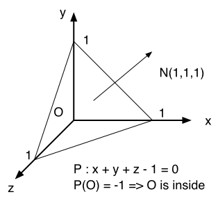
Example: Plane Equations
Orientation of a polygon ?
Often in the graphics pipeline, we need to know the orientation of an object. It would be useful to store the plane equation with the polygons so that this information doesn't have to be computed each time.
The plane equation takes the form:P(M) = Ax + By + Cz + D = 0Using any three points from a polygon, we can solve for the coefficients. Then we can use the equation to determine whether a point is on the inside or outside of the plane formed by this polygon: Ax + By + Cz + D < 0 ==> inside
|
 |
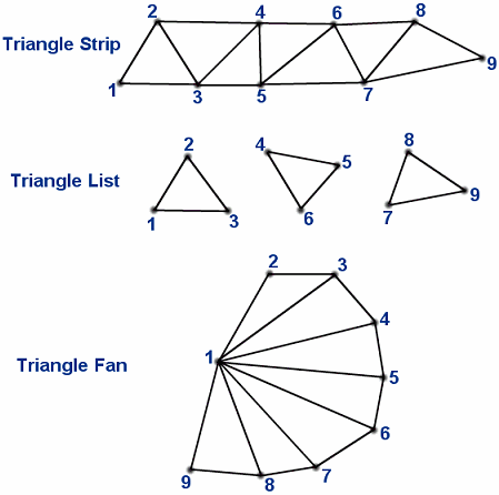
Polygon Meshes
You should break your polygon into triangle, because if you don't, your API will do it for you in a way that could not suits you (triangle renderer are implemented in hardware, especially when using gouraud shading)
The polygons we can represent can be arbitrarily large, both in terms of the number of vertices and the area. It is generally convenient and more appropriate to use a polygon mesh rather than a single mammoth polygon.
For example, you can simplify the process of rendering polygons by breaking all polygons into triangles. Then your triangle renderer from project two would be powerful enough to render every polygon. Triangle renderers can also be implemented in hardware, making it advantageous to break the world down into triangles.
Another example where smaller polygons are better is the Gouraud lighting model. Gouraud computes lighting at vertices and interpolates the values in the interiors of the polygons. By breaking larger surfaces into meshes of smaller polygons, the lighting approximation is improved.
Whenever you can, use Triangle strip, Triangle Fan, Quad StripTriangle mesh produces n-2 triangles from a polygon of n vertices.Triangle list will produce only a n/3 trianglesQuadrilateral mesh produces (n-1) by (m-1) quadrilaterals from an n x m array of vertices.Not co-planar polygonSpecifying polygons with more than three vertices could result in sets of points which are not co-planar! There are two ways to solve this problem:
|
 |
From Curves to Surfaces
Curves
Hermite
Bezier
Spline
Uniform B-Spline
Surfaces
Hermite
Bezier
B-Spline
Parametric Cubic Curves and Bicubic Patches Using Splines
bicubic surface patches.
![]()
If one parameter is held at a constant value then the
above will represent a curve. Thus P(u,a) is a curve on the surface with the
parameter v being a constant a.
In a bicubic surface patch cubic polynomials are used to represent the edge
curves P(u,0), P(u,1), P(0,v) and P(1,v)as shown below. The surface is then
generated by sweeping all points on the boundary curve P(u,0) (say) through
cubic trajectories,defined using the parameter v, to the boundary curve P(u,1).
In this process the role of the parameters u and v can be reversed.
|
 |
Beziér Patches
Control polyhedron with 16 points and the resulting bicubic patch:
The representation of the bicubic surface patch can be
illustrated by considering the Bezier Surface Patch.
The edge P(0,v) of a Bezier patch is defined by giving four control points P00,
P01, P02 and P03. Similarly the opposite edge P(1,v) can be represented by a
Bezier curve with four control points. The surface patch is generated by sweeping
the curve P(0,v) through a cubic trajectory in the parameter u to P(1,v). To
define this trajectory we need four control points, hence the Bezier surface
patch requires a mesh of 4*4 control points as illustrated above.
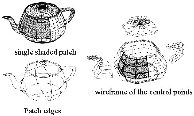
Example: The Utah Teapot
32 patches
Single shaded patch - Wireframe of the control points - Patch edges
Subdivision of Beziér Surfaces
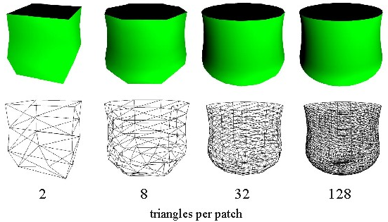
We can now apply the same basic idea to a surface, to yield increasingly accurate polygonal representations
For more, See : Rendering
Cubic Bezier Patches
by Chris Bentley
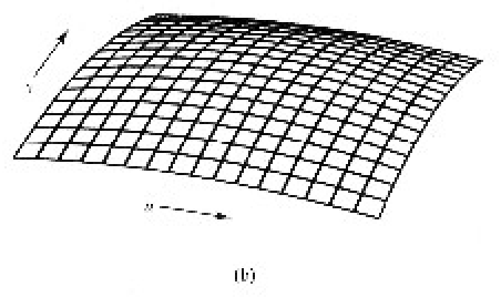
Deforming a Patch
The net of control points forms a polyhedron in cartesian space, and the positions of the points in this space control the shape of the surface.The effect of lifting one of the control points is shown on the right. |
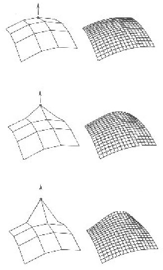 |
Patch Representation vs. Polygon Mesh
It’s fair to say that a polygon is a simple and flexible building block. However, a parametric representation of an object has certain key advantages:
Conciseness
A parametric representation is exact and economic since it is analytical. With a polygonal object, exactness can only be approximated at the expense of extra processing and database costs.
Deformation and shape change
Deformations of parametric surfaces is no less well defined than its undeformed counterpart, so the deformations appear smooth. This is not generally the case with a polygonal object.
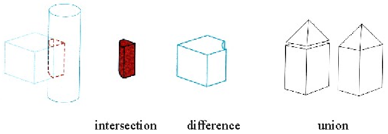
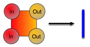
Constructive Solid-Geometry Methods (CSG)
Constructive models represent a solid as a combination of primitive solids. (CSG)
This modeling technique combine the volumes occupied by overlapping 3D shapes
using set boolean operations.
This creates a new volume by applying the union, intersection, or difference
operation to two volumes.
Each primitive is defined as a combination of half-spaces.
Typical standard primitives are:
cone, cylinder, sphere, torus, block, closed spline surface, right angular wedge.
swept solids (a revolution or linear sweep of a planar face which may
contain holes).
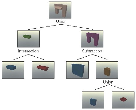
The method of Constructive Solid Geometry arose from the observation that many industrial components derive from combinations of various simple geometric shapes such as spheres, cones, cylinders and rectangular solids. In fact the whole design process often started with a simple block which might have simple shapes cut out of it, perhaps other shapes added on etc. in producing the final design. For example consider the simple solid below:
This simple component could be produced by gluing two rectangular blocks together and then drilling the hole. Or in CSG terms the the union of two blocks would be taken and then the difference of the resultant solid and a cylinder would be taken. In carrying out these operations the basic primitive objects, the blocks and the cylinder, would have to be scaled to the correct size, possibly oriented and then placed in the correct relative positions to each other before carrying out the logical operations.
The Boolean Set Operators used are:
- union - A + B is the set of points that are in A or B.
- intersection - A.B is the set of points that belong to A and B.
- difference - A-B is the set of points that belong to A but not to B.
Note that the above definitions are not rigorous and have to be refined to define the Regularised Boolean Set Operations to avoid impossible solids being generated.
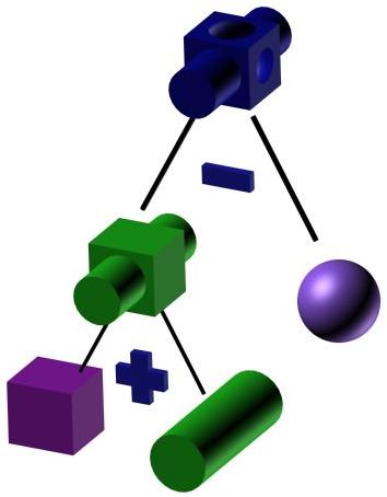
A CSG model is then held as a tree structure whose terminal nodes are primitive objects together with an appropriate transformation and whose other nodes are Boolean Set Operations. This is illustrated below for the object above which is constructed using cube and cylinder primitives.
CSG methods are useful both as a method of representation and as a user interface technique. A user can be supplied with a set of primitive solids and can combine them interactively using the boolean set operators to produce more complex objects. Editing a CSG representation is also easy, for example changing the diameter of the hole in the example above is merely a case of changing the diameter of the cylinder.
However it is slow to produce a rendered image of a model from a CSG tree. This is because most rendering pipelines work on B-reps and the CSG representation has to be converted to this form before rendering. Hence some solid modellers use a B-rep but the user interface is based on the CSG representation.
Sweep Representations
Solid modeling packages often provide a number of construction techniques. A good example is a sweep, which involves specifying a 2D shape and a “sweep” that moves the shape through a region of space.
Exemple : rotation around an axis, but it could be along any path
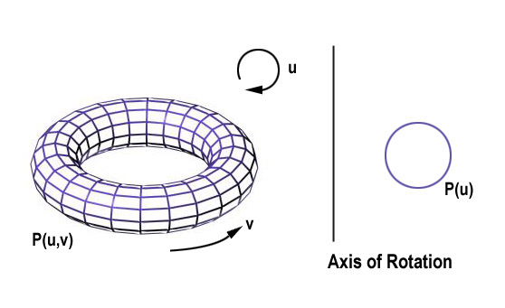 Example
of torus designed using a rotational sweep. The periodic spline cross section
is rotated about an axis of rotation specified in the plane of the cross section.
Example
of torus designed using a rotational sweep. The periodic spline cross section
is rotated about an axis of rotation specified in the plane of the cross section.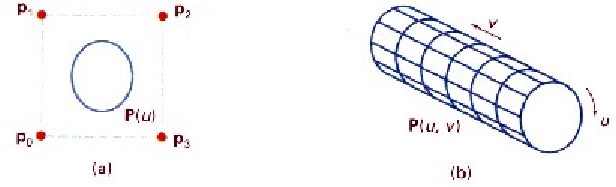
We perform a sweep by moving the shape along a path. At intervals along this path, we replicate the shape and draw a set of connectiong line in the direction of the sweep to obtain the wireframe reprensentation.
A CSG Tree Representation
Implementation with ray casting
Ray Casting is often used to implement CSG operation when objects are described with boundary representation. We fire a ray from the plane xy (which represent the screen). The surface limits for the composite object are determined by the specified set operation (see Table).
Operation |
Surface Limit |
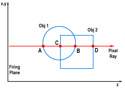 |
Union |
A, D |
|
Intersection |
C, B |
|
Difference (Obj2 - Obj1) |
B, D |
A CSG Tree Representation
Example Modeling Package: Maya
TDI, Alias WaveFront...
Volume Modeling
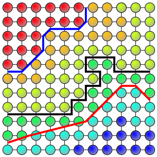
Surface-fitting Algorithms : How to draw isosurface ?
Contour Tracking / Opaque Cubes
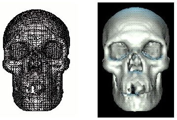
Marching Cubes Algorithm
Extracting a surface from voxel data:
|
  |
Marching Cube Cases
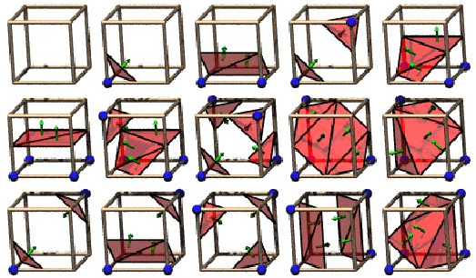
The 15 Cube Combinations
Extracted Polygonal Mesh
Metaballs
Metaballs, also known as blobby objects, are a type of implicit modeling technique. We can think of a metaball as a partical surrounded by a density field, where the density attributed to the particle (its influence) decreases with distance from the particle location. A surface is implied by taking an isosurface through this density field - the higher the isosurface value, the nearer it will be to the particle.
An Overview of Metaballs/Blobby Objects
Procedural Techniques: Fractals
Apply algorithmic rules to generate shapes
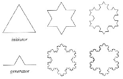
The
fractal subdivision algorithm for generating mountains
Markus Altmann
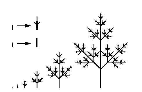
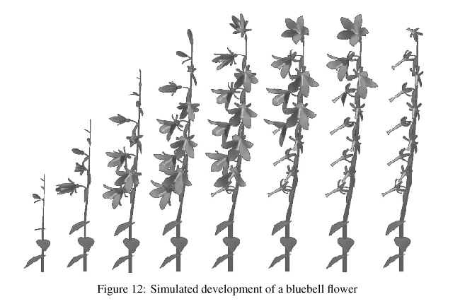
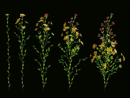
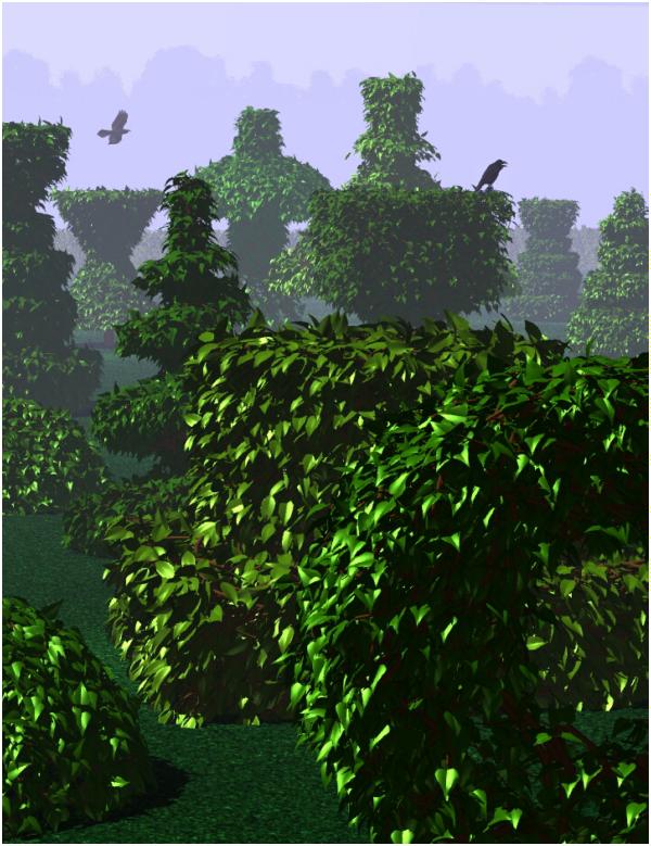
Procedural Modeling... Lindenmayer-System or L-System
Biologically-motivated approach to modeling botanical structures
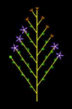
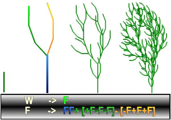
And have a look again to the 2002 first CG assignment
or "Simulating plant growth" by Marco Grubert
Physically Based Modelling Methods
Physical modelling is a way of describing the behavior of an object in terms of the interactions of external and internal forces.Simple methods for describing motion usually resort to having the object follow a pre-determined trajectory.Physical modelling, on the other hand, is about dynamics.Physically based modelling methods will tell show us how a table-cloth will drape over a table or how a curtain will fall from a window.A common method for approximating such nonrigid objects is as a network of points with flexible connections between them. |
 |
Spring Networks
A simple type of connection is a spring.
When external forces are applied, the amount of stretching or compression depends on the properties of the spring. For the simple spring, this is just the spring constant k, and the restoring force is given by F = -kx.
If the object is completely flexible, it will return to its original configuration when external forces are removed. If want to model puddy, which deforms, we would need a more complicated model of the spring.
Particle Systems
Allow us to describe natural or irregular shaped objects which are flowing or fluid-like, particular objects which are changing over time.
We can model objects, like grass, which are not actually composed of particles but which are fluid in form.
We can also model objects, like waterfalls and fireworks, which are actual physical processes that we can attempt to model through particles.
  |
Collection of particles - A particle system is composed of one or more individual particles.Stochastically defined attributes : some type of random elementPosition, Velocity (speed and direction), Color, Lifetime, Age, Shape, Size, TransparencyParticle Life CycleGeneration - Particles in the system are generated randomly within a predetermined location of the fuzzy objectParticle Dynamics - The attributes of each of the particles may vary over time. (particle position is going to be dependent on previous particle position and velocity as well as timeExtinction - Each particle has two attributes dealing with length of existence: age and lifetime.Rendering |
Example : 
Extract from : Particle Systems by Allen Martin
The term particle system is loosely defined in computer graphics. It has been used to describe modeling techniques, rendering techniques, and even types of animation. In fact, the definition of a particle system seems to depend on the application that it is being used for. The criteria that hold true for all particle systems are the following:
Collection of particles - A particle system is composed of one or more individual particles. Each of these particles has attributes that directly or indirectly effect the behavior of the particle or ultimately how and where the particle is rendered. Often, particles are graphical primitives such as points or lines, but they are not limited to this. Particle systems have also been used to represent complex group dynamics such as flocking birds.
Stochastically defined attributes - The other common characteristic of all particle systems is the introduction of some type of random element. This random element can be used to control the particle attributes such as position, velocity and color. Usually the random element is controlled by some type of predefined stochastic limits, such as bounds, variance, or type of distribution.
Each object in Reeves particle system had the following
attributes:
Position
Velocity (speed and direction)
Color
Lifetime
Age
Shape
Size
Transparency
Particle Life Cycle
Each particle goes through three distinct phases in the particle system: generation,
dynamics, and death. These phases are described in more detail here:
Generation - Particles in the system are generated randomly within a predetermined
location of the fuzzy object. This space is termed the generation shape of the
fuzzy object, and this generation shape may change over time. Each of the above
mentioned attribute is given an initial value. These initial values may be fixed
or may be determined by a stochastic process.
Particle Dynamics - The attributes of each of the particles may vary over time.
For example, the color of a particle in an explosion may get darker as it gets
further from the center of the explosion, indicating that it is cooling off.
In general, each of the particle attributes can be specified by a parametric
equation with time as the parameter. Particle attributes can be functions of
both time and other particle attributes. For example, particle position is going
to be dependent on previous particle position and velocity as well as time.
Extinction - Each particle has two attributes dealing with length of existence:
age and lifetime. Age is the time that the particle has been alive (measured
in frames), this value is always initialized to 0 when the particle is created.
Lifetime is the maximum amount of time that the particle can live (measured
in frames). When the particle age matches it's lifetime it is destroyed. In
addition there may be other criteria for terminating a particle prematurely:
Running out of bounds - If a particle moves out of the viewing area and will
not reenter it, then there is no reason to keep the particle active.
Hitting the ground - It may be assumed that particles that run into the ground
burn out and can no longer be seen.
Some attribute reaches a threshold - For example, if the particle color is so
close to black that it will not contribute any color to the final image, then
it can be safely destroyed.
Rendering
When rendering this system of thousands of particles, some assumptions have
to be made to simplify the process. First, each particle is rendered to a small
graphical primitive (blob). Particles that map to the same pixels in the image
are additive - the color of a pixel is simply the sum of the color values of
all the particles that map to it. Because of this assumption, no hidden surface
algorithms are needed to render the image, the particles are simply rendered
in order. Effects like temporal ant-aliasing (motion blur) are made simple by
the particle system process. The position and velocity are known for each particle.
By rendering a particle as a streak, motion blur can be achieved.