eScience Lectures Notes : Illumination and Shading
Slide 1 : 1 / 32 : Illumination and Shading
Illumination and Shading
Slide 2 : Illumination and Shading
Illumination and Shading
Light Sources
Empirical Illumination
Shading
Transforming Normals
Slide 3 : 3 / 32 : Illumination Models
Illumination Models
Computer Graphics Jargon:
-
Illumination - the transport of luminous flux from light sources
between points via direct and indirect paths
-
Lighting - the process of computing the luminous intensity reflected
from a specified 3-D point
-
Shading - the process of assigning a colors to a pixels
|
 |
Illumination Models:
-
Empirical : simple formulations that approximate observed
phenomenon
Java3D : Real Time illumination model : lots of
approximations. No Shade, simplified transparency, no reflexion (miror).
OpenGL, SGI trick : two time the same scene to simulate
real time reflexion on the floor.
-
Physically-based : models based on the actual physics of light's
interactions with matter
Raytracing, Radiosity...
-
Local illumination model / Global illumination model
|
From Physics we can derive models, called "illumination
models", of how light reflects from surfaces and produces what we perceive
as color. In general, light leaves some light source, e.g. a lamp or the sun,
is reflected from many surfaces and then finally reflected to our eyes, or through
an image plane of a camera.
The contribution from the light that goes directly from
the light source and is reflected from the surface is called a "local illumination
model". So, for a local illumination model, the shading of any surface
is independent from the shading of all other surfaces.
A "global illumination model" adds to the local
model the light that is reflected from other surfaces to the current surface.
A global illumination model is more comprehensive, more physically correct,
and produces more realistic images. It is also more computationally expensive.
We will first look at some basic properties of light and color, the physics
of light-surface interactions, local illumination models, and global illumination
models.
Scan-line rendering methods use only local illumination
models, although they may use tricks to simulate global illumination. Many current
graphics images and commercial systems are in this category, but many systems
are becoming global illumination based.
The two major types of graphics systems that use global
illumination models are radiosity and ray tracing. These produce more realistic
images but are more computationally intensive than scan-line rendering systems.
Slide 4 : 4 / 32 : Two Components of Illumination
Two Components of Illumination
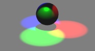
Every object in a scene is potentially a source of light.
Light may be either be emitted or reflected from objects. Generally, in computer
graphics we make a distinction between light emitters and light reflectors.
The emitters are called light sources, and the reflectors are usually the objects
being rendered. Light sources are characterized by their intensities while reflectors
are characterized by their material properties.
Light Sources
-
Emittance Spectrum (color)
-
Geometry (position and direction)
-
Directional Attenuation
Surface Properties
-
Reflectance Spectrum (color)
for different aspects of illumination
-
Geometry (position, orientation, and micro-structure)
-
Absorption
|
|
Simplifications used by most real time scomputer graphics
systems:
-
Only the direct illumination from the emitters to the reflectors
of the scene
-
Ignore the geometry of light emitters, and consider only the geometry
of reflectors
-
most of the light from a scene results from a single bounce of a
emitted ray off of a reflective surface
Most computer graphic rendering systems only attempt
to model the direct illumination from the emitters to the reflectors of
the scene. On the other hand most systems ignore the geometry of light
emitters, and consider only the geometry of reflectors. The rationalization
behind these simplifications is that most of the light from a scene results
from a single bounce of a emitted ray off of a reflective surface. This
is, however, a very questionable assumption. In most computer generated
pictures you will not see light directly emitted from the light source,
nor the indirect illumination from a light reflecting off on surface and
illuminating another. |
Things forgotten or oversimplified here |
-
Polarisation
-
Index of refraction of material (variation fonction of wavelength)
|
-
Difraction
-
Surface evolution
|
First we will consider some very simple lighting models.
Slide 5 : 5 / 32 : Ambient Light Source
Ambient Light Source
On earth, an object is still visible even if not directlty lit
Even though an object in a scene is not directly lit it will still be visible.
This is because light is reflected indirectly from nearby objects. A simple
hack that is commonly used to model this indirect illumination is to use of
an ambient light source.
Ambient Ligth source : no spatial or directional characteristics
-
The amount of ambient light incident on each object is a constant for
all surfaces in the scene.
-
An ambient light can have a color.
-
The amount of ambient light that is reflected by an object is independent
of the object's position or orientation.
-
Surface properties are used to determine how much ambient light is reflected.
The look of a scene with only Ambient Light Source is
very flat
Ambient light is the illumination of an object caused by reflected light from
other surfaces. To calculate this exactly would be very complicated. A simple
model assumes ambient light is uniform in the environment.
Slide 6 : 6 / 32 : Directional Light Sources
 Directional
Light Sources
Directional
Light Sources
-
 All
of the rays from a directional light source have the same direction, and
no point of origin.
All
of the rays from a directional light source have the same direction, and
no point of origin.
-
It is as if the light source was infinitely far away from the surface
that it is illuminating.
-
Sunlight is an example of an infinate light source.
Involved in Diffuse and Specular components of illumination.
We consider the direction of the light source when computing
both the diffuse and specular components of illumination.
With a directional light source this direction is a constant.
Slide 7 : 7 / 32 : Point Light Sources
Point Light Sources
The rays emitted from a point light radially diverge from the source.
A point light source is a fair approximation to a local light source
such as a light bulb.
The direction of the light to each point on a surface changes when a
point light source is used.
Thus, a normalized vector to the light emitter must be computed for each
point that is illuminated.
|
|
|
|
|
Slide 8 : 8 / 32 : Other Light Sources
Other Light Sources
Slide 9 : 9 / 32 : Ideal Diffuse Reflection
Ideal Diffuse Reflection ...
...On a ideal diffuse reflector : a very rough surface.
First, we will consider a particular type of surface
called an ideal diffuse reflector. An ideal diffuse surface is, at
the microscopic level, a very rough surface.
Chalk is a good approximation to an ideal diffuse surface.
Because of the microscopic variations in the surface, an incoming ray
of light is equally likely to be reflected in any direction over the hemisphere.
|
|
Diffuse reflections are constant over each surface in
a scene, independent of the viewing direction.
Slide 10 : 10 / 32 : Lambert's Cosine Law
Lambert's Cosine Law
Ideal diffuse reflectors = Lambertian reflectors
Ideal diffuse reflectors reflect light according to Lambert's
cosine law, (these are sometimes called Lambertian reflectors).
Law : reflected energy from a small surface area in a particular direction
is proportional to the cosine of the angle between that direction and the surface
normal
Lambert's law states that the reflected energy from a
small surface area in a particular direction is proportional to the cosine of
the angle between that direction and the surface normal. Lambert's law determines
how much of the incoming light energy is reflected.
Reflected intensity is independent of the viewing direction, but dependent
of the source orientation.
Remember that the amount of energy that is reflected in
any one direction is constant in this model. In other words, the reflected intensity
is independent of the viewing direction.
The intensity does, however, depend on the light source's
orientation relative to the surface, and it is this property that is governed
by Lambert's law.
Slide 11 : 11 / 32 : Computing Diffuse Reflection
Computing Diffuse Reflection
Angle of Incidence
The angle between the surface normal and the incoming
light ray is called the angle of incidence and we can express a intensity of
the light in terms of this angle.
The Ilight term represents the intensity
of the incoming light at the particular wavelength (the wavelength determines
the light's color). The kd term represents
the diffuse reflectivity of the surface at that wavelength.
Vector use
In practice we use vector analysis to compute cosine term indirectly. If both
the normal vector and the incoming light vector are normalized
(unit length) then diffuse shading can be computed as follows:
Slide 12 : 12 / 32 : Diffuse Lighting Examples
Diffuse Lighting Examples
We need only consider angles from 0 to 90 degrees.
Greater angles (where the dot product is negative) are blocked by the surface,
and the reflected energy is 0.
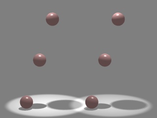
Below are several examples of a spherical diffuse reflector
with a varying lighting angles.
Why do you think spheres are used as examples when shading?
What is missing ??? a little shiny spot ?
Slide 13 : 13 / 32 : Specular Reflection
Specular Reflection
Specular reflector : Shiny surface : Very smooth surface
A second surface type is called a specular reflector.
When we look at a shiny surface, such as polished metal or a glossy car finish,
we see a highlight, or bright spot. Where this bright spot appears on the surface
is a function of where the surface is seen from. This type of reflectance is
view dependent.
At the microscopic level a specular reflecting surface
is very smooth, and usually these microscopic surface elements are oriented
in the same direction as the surface itself.
Ideal mirror : a purely specular reflector
Specular reflection is merely the mirror reflection of
the light source in a surface. Thus it should come as no surprise that it is
viewer dependent, since if you stood in front of a mirror and placed your finger
over the refelection of a light, you would expect that you could reposition
your head to look around your finger and see the light again. An ideal mirror
is a purely specular reflector.
In order to model specular reflection we need to understand
the physics of reflection.
Slide 14 : 14 / 32 : Snell's Law
Snell's Law (1636 Snell discovers Descarte's laws...)
Reflection behaves according to Snell's laws which
state:
One common Plane
The incoming ray, the surface normal, and the reflected
ray all lie in a common plane.
One relation between angle
The angle that the reflected ray forms with the
surface normal is determined by the angle that the incoming ray forms
with the surface normal, and the relative speeds of light of the mediums
in which the incident and reflected rays propogate according to the following
expression.
|
DESCARTE'S DIOPTRICS, 1637
Reflection : a special case of the law
Reflection is a very special case of Snell's Law
where the incident light's medium and the reflected rays medium is the
same. Thus we can simplify the expression to:

|
1620s: Snell and Descarte, Snell’s Law : http://www.geo.hunter.cuny.edu/~afrei/theory_of_light_lecture.htm
SNELL'S LAW (FROM DESCARTE'S DIOPTRICS, 1637) : http://bayes.cs.ucla.edu/LECTURE/lecture_sec1.htm
1636 Snell discovers Descarte's laws... : unix.temple.edu/~meziani/history.pdf
Snell deduced his law from experimental data and thought
that cosecants fitted his data best. The frenchman Descarte was the first to
use the correct sines. In France it is known as Descarte's Law! http://www.star.le.ac.uk/~rw/courses/lect220.html
Slide 15 : 15 / 32 : Non-ideal Reflectors
Non-ideal Reflectors
Real material, other than mirrors and chrome
Snell's law, however, applies only to ideal mirror reflectors.
Real materials, other than mirrors and chrome tend to deviate significantly
from ideal reflectors. At this point we will introduce an empirical model
that is consistent with our experience, at least to a crude approximation.
Empirical model
-
microscopic surface variations
-
light just slightly offset from the ideal reflected ray
In general, we expect most of the reflected light to
travel in the direction of the ideal ray. However, because of microscopic
surface variations we might expect some of the light to be reflected just slightly
offset from the ideal reflected ray. As we move farther and farther, in the
angular sense, from the reflected ray we expect to see less light reflected.
Slide 16 : 16 / 32 : Phong Illumination
Phong Illumination model
-
One function that approximates this fall
-
No Physical basis, but very successful
One function that approximates this fall off is called
the Phong Illumination model. This model has no physical basis, yet it is one
of the most commonly used illumination models in computer graphics.
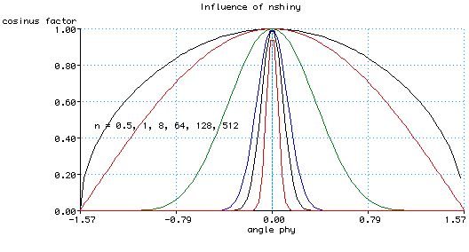
The cos f term is maximum when
the surface is viewed from the mirror direction and falls off to 0 when viewed
at 90 degrees away from it. The nshiny term controls
the rate of this fall off.
Note that this equation is only valid for f
< PI/2
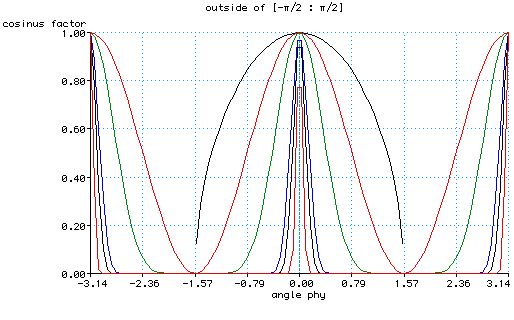
Slide 17 : 17 / 32 : Effect of nshiny
Effect of nshiny
The diagram below shows the how the Phong reflectance
drops off based on the viewers angle from the reflected ray for various values
of nshiny.
Slide 18 : 18 / 32 : Computing Phong Illumination
Computing Phong Illumination
Another formulation
The cos term of Phong's specular illumination could be
replaced using the following relationship.
-
V : Viewer unit vector
-
R : mirror Reflectance unit vector
The V vector is the unit vector in the direction
of the viewer and the R vector is the mirror reflectance direction.
The vector R can be computed from the incoming
light direction and the surface normal as shown below.
The following figure illustrates this relationship.
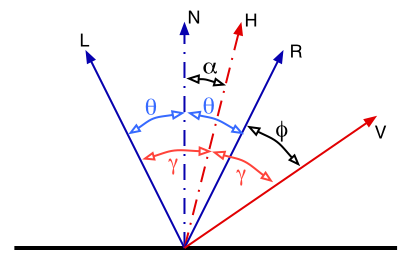
Slide 19 : 19 / 32 : Blinn & Torrance Variation
Blinn & Torrance Variation
Jim Blinn introduced another approach for computing Phong-like illumination
based on the work of Ken Torrance.
His illumination function uses the following equation:
In this equation the angle of specular dispersion is computed by how far the
surface's normal is from a vector bisecting the incoming light direction and
the viewing direction.
q + f = a +
g q + a
= g =>
f - a = a
f = 2a
On your own you should consider how this approach and
the previous one differ.
N : Normal to the real plan
H : Normal to the plane that would create higher reflexion
towards the viewer
Advantage : the angle (N,H) will always remains between
0 and PI/2
Careful : nshiny should introduce a factor 2 with the
previous expression.
Slide 20 : 20 / 32 : Phong Examples
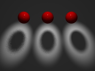
Phong Examples
The following spheres illustrate specular reflections
as the direction of the light source and the coefficient of shineyness is varied.
Influence of the illumination...
compared to the diffuse model...
Slide 21 : 21 / 32 : Summary of 3 Illumination Models
Summary of 3 Illumination Models
Illumination models take into account each individual
point on a surface and the light sources that are directly illuminating it.
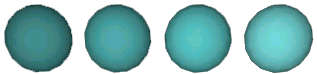
Ambient Reflection
Ambient reflection is the result of inter-reflection from
the walls and objects. However, it is modelled as a constant term for the specific
object, such that a 3D sphere looks 2D. This approximates diffuse reflection
globally.

Spheres shaded showing variation of magnitude in ambient
component over the surface of each sphere. From left to right, increasing amount
of cyan ambient reflection.
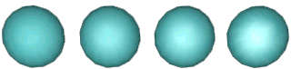
Diffuse Reflection
Most objects around us do not emit light of their own.
Rather they absorb daylight, or light emitted from an artificial source, and
reflect part of it. Here, light that reached the surfaces would be scattered
equally in all directions. This implies that the amount of light as observed
by the viewer is independent of the viewer's location.
Spheres shaded showing variation of magnitude in diffuse
component over the surface of each sphere. From left to right, increasing amount
of cyan diffuse reflection.
Specular Reflection
Many real world surfaces are glossy, such that when viewed
from certain angles they can be seen reflecting light. A glossy surface reflects
a high proportion of light, while the rest is the result of diffuse reflection.
This glossy or shiny reflection is called specular reflection.
Spheres shaded showing variation of magnitude in specular
component over the surface of each sphere. From left to right, increasing amount
of specular reflection.
Slide 22 : 22 / 32 : Putting it all together
Putting it all together : Local Illumination Summary
Our final empirical illumination model is:
|
Notes:
-
The Phong Lighting model
-
Once per light
-
Once per color component
-
Reflectance coefficients fonction of color
Reflectance coefficients, ka, kd, and ks may or
may not vary with the color component
If they do, you need to be careful.
|
 |
Slide 23 : 23 / 32 : What else about illumination ?
What else about illumination ?
Warn model
Control of the intensity with reagards of the direction of a spot light.
Light sources are modeled as points on a reflecting surface, using the Phong
model.
Intensity Attenuation
attenuation function applied to point light source
f(d) = 1/(a0 + a1.d + a2.d^2)
where d is the distance between the source and the illuminated surface
Transparency
In Real Time API, a rough approximation with a percentage of refraction light.
no shifting of the path
Ò
Slide 24 : 24 / 32 : Where do we Illuminate ?
Where do we Illuminate ?...
From Illumination (a costly process), lighting model to...
To this point we have discussed how to compute an illumination
model at a point on a surface.
But, at which points on the surface is the illumination
model applied? Where and how often it is applied has a noticable effect on the
result.
Illuminating can be a costly process involving the
computation of and normalizing of vectors to multiple light sources and the
viewer.
... Shading or Surface rendering algorithm
For models defined by collections of polygonal facets or triangles:
-
Each facet has a common surface normal
-
If the light is directional then the diffuse contribution is constant
across the facet
-
If the eye is infinitely far away and the light is directional then the
specular contribution is constant across the facet
Slide 25 : 25 / 32 : Flat Shading
Constant or Flat Shading
One illumination calculation for each facet/polygon
The simplest shading method applies only one illumination
calculation for each primitive. This technique is called constant or flat shading.
It is often used on polygonal primitives.
Computation done at the centroid
Illumination is computed for only a single point on the facet.
Which one? Usually the centroid. For a convex facet the centriod is given as
follows:
Issues:
For point light sources the direction to the light source varies over the
facet
For specular reflections the direction to the eye varies over the facet
Slide 26 : 26 / 32 : Facet Shading
Facet Shading
This shading is just a working hypothesis, that is not
usually used
Even when the illumination equation is applied at each point of the faceted
nature of the polygonal nature is still apparent. The issue is the dicontinuity
of normals !
To overcome this limitation normals are introduced at each vertex.
-
Usually different than the polygon normal
-
Used only for shading (not backface culling or other geometric computations)
-
Better approximates the "real" surface
-
Assumes the polygons were a piecewise approximation of the real surface
(C0)
-
Normals provide information about the tangent plane at each point (C1)
-
Usually the average of the tangent of the neighbour facets
- not always (real discontinuity or more straightforwards value (sphere for
instance).
Slide 27 : 27 / 32 : Vertex Normals
Vertex Normals
If vertex normals are not provided they can often be approximated by averaging
the normals of the facets which share the vertex.
This only works if the polygons reasonably approximate
the underlying surface.
 A
better approximation can be found using a clustering analysis of the normals
on the unit sphere.
A
better approximation can be found using a clustering analysis of the normals
on the unit sphere.
Slide 28 : 28 / 32 : Triangle Normals
Triangle Normals
Now that we understand the geometric implications of a
normal it is easy to figure out how to transform them.
On a facetted planar surface vectors in the tangent plane can be computed using
surface points as follows. Normals are always orthogonal to the tangent space
at a point. Thus, given two tangent vectors we can compute the normal as follows:This
normal is perpendicular to both of these tangent vectors.
Slide 29 : 29 / 32 : Normals of Nonplanar Surfaces
Normals of non planar Surfaces
Example : parametric surface
Not all surfaces are given as planar facets. A common
example of such a surface is called a parametric surface. For a parametric surface
the three-space coordinates are determined by functions of two parameters, u
and v in our case. For parametric surfaces two vectors in the tangent plane
can be found by computing partial derivatives as follows. And the normal is
computed as before:
Slide 30 : 30 / 32 : Gouraud Shading
Gouraud Shading
Interpolation of the intensity
The Gouraud Shading method applies the illumination model on a subset of surface
points and interpolates the intensity of the remaining points on the surface.
In the case of a polygonal mesh the illumination model is usually applied
at each vertex and the colors in the triangles interior are linearly interpolateded
from these vertex values.

The linear interpolation can be accomplished using the plane equation method
discussed in the lecture on rasterizing polygons.
Notice that facet artifacts are still visible.
Gouraud shading is by no means perfect, but it can make a real difference
over flat shaded polygons. Problems with Gouraud shading occur when you try
to mix light sourcing calculations with big polygons.
Imagine you have a large polygon, lit by a light near
it's center. The light intensity at each vertex will be quite low, because they
are far from the light. The polygon will be rendered quite dark, but this is
wrong, because it's centre should be brightly lit. You can see this happening
in the game Descent. Firing flares around, especially into corners, causes the
surroundings to light up. But try firing a flare into the middle of a large
flat wall or floor, and you will see that it has very little effect.
However, if you are using a large number of small polygons, with a relatively
distant light source, Gouraud shading can look quite acceptable. Infact, the
smaller the polygons, the closer it comes to Phong shading.
Gouraud Shading: Named after its inventor, Henri Gouraud
who developed this technique in 1971 (yes, 1971). It is by far the most common
type of shading used in consumer 3D graphics hardware, primarily because of
its higher visual quality versus its still-modest computational demands. This
technique takes the lighting values at each of a triangle's three vertices,
then interpolates those values across the surface of the triangle. Gouraud shading
actually first interpolates between vertices and assigns values along triangle
edges, then it interpolates across the scan line based on the interpolated edge
crossing values. One of the main advantages to Gouraud is that it smoothes out
triangle edges on mesh surfaces, giving objects a more realistic appearance.
The disadvantage to Gouraud is that its overall effect suffers on lower triangle-count
models, because with fewer vertices, shading detail (specifically peaks and
valleys in the intensity) is lost. Additionally, Gouraud shading sometimes loses
highlight detail, and fails to capture spotlight effects.
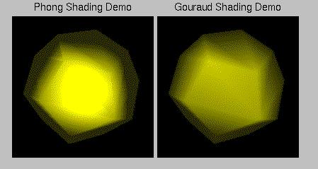
Slide 31 : 31 / 32 : Phong Shading
Phong Shading
-
Not to be confused with Phong illumination model
-
Linear interpolation of the surface normals
-
Illumination model applied at every point
In Phong shading (1975 - Phong Biu-Tuong)(not to be confused
with Phong's illumination model), the surface normal is linearly interpolated
across polygonal facets, and the Illumination model is applied at every point.
A Phong shader assumes the same input as a Gouraud shader, which means that
it expects a normal for every vertex. The illumination model is applied at every
point on the surface being rendered, where the normal at each point is the result
of linearly interpolating the vertex normals defined at each vertex of the triangle.
Phong shading will usually result in a very smooth appearance, however, evidence
of the polygonal model can usually be seen along silhouettes.

 In
the Phong method, vector interpolation replaces intensity interpolation.
In
the Phong method, vector interpolation replaces intensity interpolation.
Graphic courtesy of Watt.
Slide 32 : 32 / 32 : Summary of 3 Shading Models
Summary of 3 Shading Models
There are three traditional shading models, namely flat
shading, Gouraud shading and Phong shading. Global illumination shading models
such as recursive ray tracing and radiosity takes into account the interchange
of light between all surfaces.
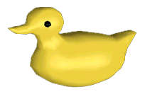
Flat Shading
Flat surface rendering or constant shading is the simplest
rendering format that involves some basic surface properties such as colour
distinctions and reflectivity. This method produces a rendering that does not
smooth over the faces which make up the surface. The resulting visualization
shows an object that appears to have surfaces faceted like a diamond.
Rendering only requires the computation of a colour for
each visible face. The whole face is
filled with this colour.
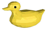
Toy duck using flat shading.
This approach is fast and very simple, but it gives quite
unrealistic results and non-smooth surfaces. This is highlighted by the Mach
effect: the intensity at the vicinities of the edges is overestimated for light
values and underestimated for dark values.
Gouraud Shading
The Gouraud shading [Gouraud, 1971] is restricted to the
diffuse component of the illumination
model and it gives a fairly realistic result
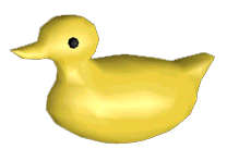
Toy duck usingGouraud shading.
It is noted that most VR systems, including Leeds Advanced
Driving Simulator and arcade
games such as Sega's Street Fighter, use Gouraud shading extensively.
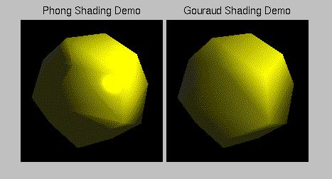
Phong Shading
Phong shading overcomes the limitation of Gouraud shading
by incorporating specular reflection
into the scheme [Phong, 1975]. Now, we have the effect of specular highlight
in the middle of
each polygon. Also note that the intensity transition from one polygon to another
is smoother.
Toy duck using Phong shading.
However, the primary objective is for efficiency of computation
rather than for accurate physical simulation. As mentioned by Phong: "We
do not expect to be able to display the object exactly as it would appear
in reality, with texture, overcast shadows, etc. We hope only to display an
image that approximates the real object closely enough to provide a certain
degree of realism."
In both shading, the Phong illumination model is applied...or
not