|
|
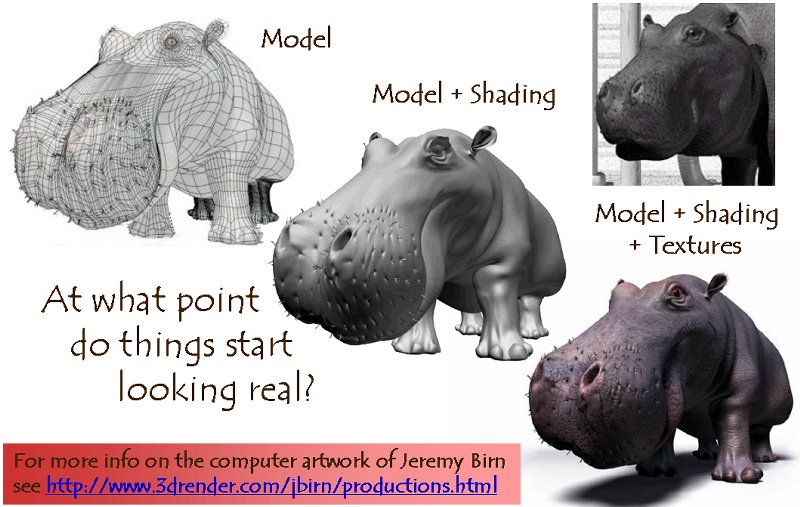
The appearance of many real world objects depends on its texture. The texture of an object is really the relatively fine geometry at the surface of an object. To appreciate the role surface textures play in the appearance of real world objects, consider carpet. Even when all of the fibers of a carpet are the same color the carpet does not appear as a constant color due to the interaction of the light with geometry of the fibers. Even though Java 3D is capable of modeling the geometry of the individual carpet fibers, the memory requirements and rendering performance for a room size piece of carpet modeled to such detail would make such a model useless. On the other hand, having a flat polygon of a single color does not make a convincing replacement for the carpet in the rendered scene.
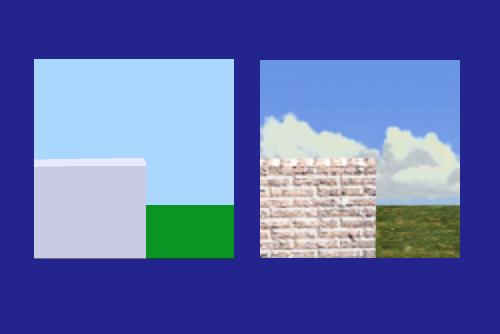
When creating image detail, it is cheaper to employ mapping techniques that it is to use myriads of tiny polygons. The image on the right portrays a brick wall, a lawn and the sky. In actuality the wall was modeled as a rectangular solid, and the lawn and the sky were created from rectangles. The entire image contains eight polygons. Imagine the number of polygon it would require to model the blades of grass in the lawn! Texture mapping creates the appearance of grass without the cost of rendering thousands of polygons.
Ed Catmull, who later founded Pixar, was sitting in his car in the parking lot of the engineering building at the University of Utah in 1974 thinking about how to make a more realistic computer animation of a castle. The problem was that modeling the rough stone walls would require prohibitively many polygons. Even if he were only interested in the color variation, not the geometric variation (bumpiness), it would still require a new polygon for each point that had a different color.
What approach would you take? He concluded that if pictures of the stone wall could be stored for reference and then be applied or mapped onto the otherwise smoothly shaded polygon, then the result would be increased scene detail without increasing geometric complexity (and its associated increased difficulty in modeling the scene).
In effect, texture mapping simply takes an image (a texture map) and wallpapers it onto the polygons in the scene.
Since those days, texture mapping has become the most important method of increasing the level of detail of a scene without increasing its geometric complexity (the number of geometric primitives in the scene).
|
 |
 |
|
Rectangular Patern Array |
|
Surface |
|
Pixel Area |
Texture Space : (s, t) Array Coordinates |
<< ====== >> |
Object Space : (u, v) Surface Parameters |
<< ====== >> |
Image Space : (x, y) Pixel Coordinates |
|
|
Texture - Surface Transformation |
|
Viewing and projection Transformation |
|
u = fu(s,t) = aus + but + cu v = fv(s,t) = avs + bvt + cv |
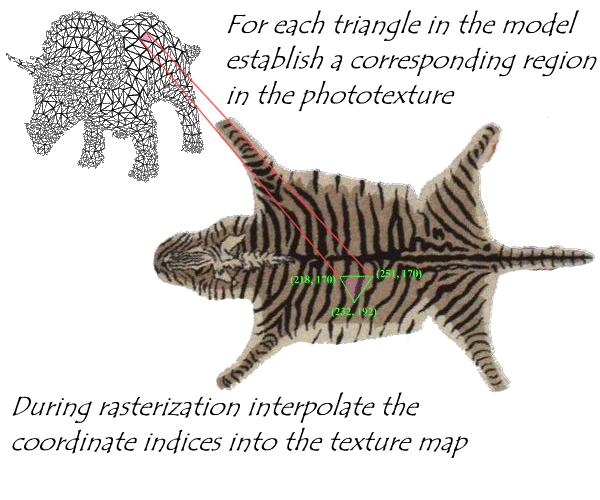
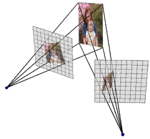
The basic method of texture mapping is to specify the coordinates in the texture map (s,t) that map to a particular point on the geometric surface. For polygonal models, the (s,t) coordinates are specified at the polygon vertices and are interpolated across the surface as are R,G,B,A,Z and other things to come. Normally, the texture coordinates are on the range [0..1] in u and v. However, for textures that are to repeat more than once going across the polygon, texture coordinates outside the [0..1] range need to be acceptable.
2D Texture Space |
3D Object Space |
3D World Space |
3D Camera Space |
2D Image Space |
|||||
|
|
Parametrization |
Model Transformation |
Viewing Transform |
Projection |
|
||||
|
|
|||||||||
Texture Scanning, Direct mapping |
============================>>> |
||||||||
<<<============================ |
Inverse Scanning,
|
||||||||
Inverse scanning is used most of the time...
Forward mapping is stepping through the texture map and computing the screen location of each texel. This is done in real-time video effects systems. Most other systems use inverse mapping, which is done by stepping through the screen pixels and computing the color of each by determining which texels map to this pixel.
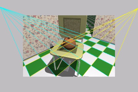
A disadvantage of mapping from texture space to pixel space is that a selected texture patch usually does not match up with the pixels boundaries, thus requiring calculation of the fractional area of pixel coverage. Therefore, mapping from pixel space to texture space is the most commonly used texture mapping method. This avoid pixel subdivision calculations and allows antialiasing (filtering) procedures to be easily applied.
Since there will almost never be a 1 to 1 mapping between pixels in the texture map (texels) and pixels on the screen, we must filter the texture map when mapping it to the screen. The way in which we accomplish the filtering depends on whether we are forward mapping or inverse mapping.
Source : Teaching Texture Mapping Visually by Rosalee Wolfe / DePaul University / wolfe@cs.depaul.edu
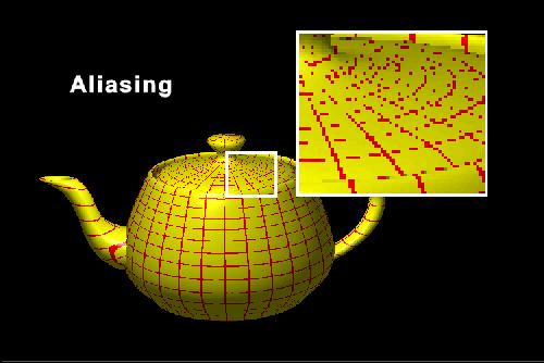
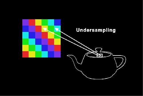
No matter the type of mapping we’re undertaking, we run the danger of aliasing. Aliasing can ruin the appearance of a texture-mapped object. Aliasing is caused by undersampling. Two adjacent pixels in an object may not map to adjacent pixels in the texture map. As a result, some of the information from the texture map is lost when it is applied to the object.
Source : Teaching Texture Mapping Visually by Rosalee Wolfe / DePaul University / wolfe@cs.depaul.edu
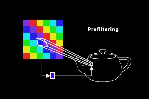
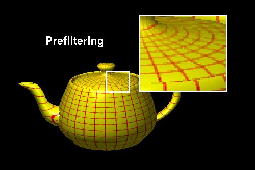
Antialiasing minimizes the effects of aliasing. One method, called prefiltering, treats a pixel on the object as an area (Catmull, 1978). It maps the pixel’s area into the texture map. The average color is computed from the pixels inside the area swept out in the texture map.
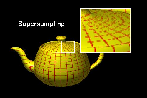
A second method, called supersampling, also computes an average color (Crow, 1981). In this example each of four corners of an object pixel are mapped into the texture. The four pixels from the texture map are averaged to produce the final color for the object.
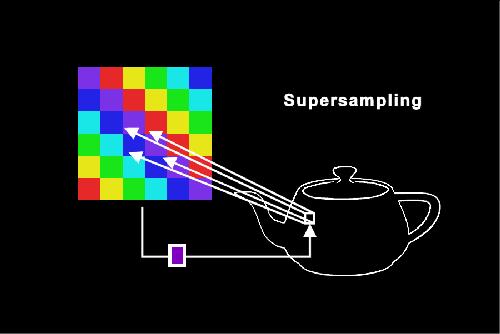
Prefiltering |
Supersampling |
 |
 |
Since many texels will probably map to each pixel, it would be extremely expensive to perform the entire filter computation at each pixel, each frame. MIP-mapping (Multum in Parvo, or many in a small place) pre-computes part of the filter operation by storing down-sampled replicas of each texture, going from the original m x n texture map all the way to a 1 x 1 texture map. At run time, if a given screen pixel maps to many texels, we simply choose the appropriate MIP-map level in which a single texel represents all the desired texels, and perform our texture sampling on that level.
Since the pixel will project to an arbitrary place on the MIP-map image, rather than exactly onto a texel, we can use bilinear or other filtering to interpolate nearby texels. This is Bilinear MIP-mapped Texture Filtering talked about in video game hardware. Better than this, we can bilinearly filter on the two most appropriate MIP-map levels and then blend the results. This is Trilinear MIP-mapped Texture Filtering. It requires the use of eight texels, and requires seven linear interpolations, but provides an important improvement over bilinear filtering.
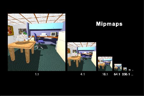
Antialiasing is expensive due to the additional computation required to compute an average color. Mipmapping saves some expense by precalculating some average colors (Williams, 1983). The mipmap algorithm first creates several versions of the texture. Beginning with the original texture the mipmap algorithm computes a new texture that’s one fourth the size. In the new, smaller texture map, each pixel contains the average of four pixels from the original texture. The process of creating smaller images continues until we get a texture map containing one pixel. That one pixel contains the average color of the original texture map in its entirety.
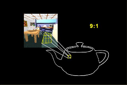
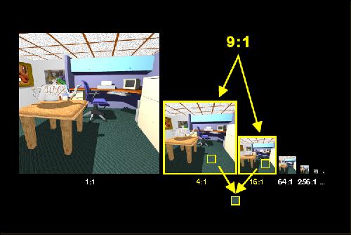
In the texture mapping phase the area of each pixel on the object is mapped into the original texture map. The mipmap computes a measure of how many texture pixels are in the area defined by the mapped pixel. In this example approximately nine texture pixels will influence the final color so the ratio of texture pixels to object pixel is 9:1.
To compute the final color, we find the two texture maps whose ratios of texture pixels are closest to the ratio for the current object pixel. We look up the pixel colors in these two maps and average them.
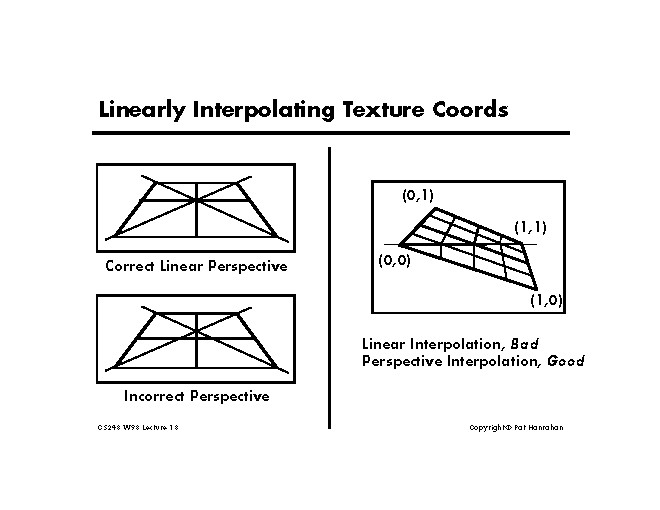
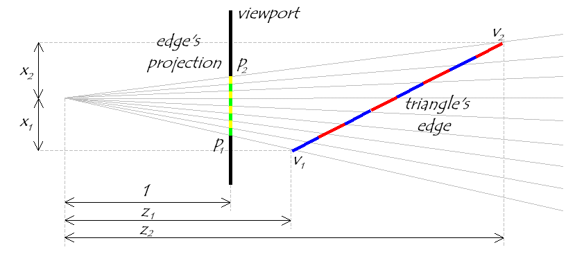
In order to correctly interpolate texture
coordinates under perspective we must consider the set of all values that will
be projected to be a single homogeneous vector:
(x, y, z, w, u, v, 1, R, G, B, A)
After transforming the vertex we have:
(xw, yw, zw, w, u, v, 1, R, G, B, A)
When projecting a homogenous vector we divide by the homogenous coordinate:
(xw/w, yw/w, zw/w, w/w, u/w, v/w, 1/w, R/w, G/w, B/w, A/w)
We then interpolate between the vertices and perform the projection of the texture
coordinates at the pixels. That is, at the vertices we compute u/w, v/w, and
1/w. We linearly interpolate these three across the pixels. Then at each pixel
we divide the interpolated texture coordinates by the interpolated 1/w to yield
the final u,v.
For more information about that issue, see : http://easyweb.easynet.co.uk/~mrmeanie/tmap/tmap.htm
Source : http://graphics.stanford.edu/courses/cs248-98-fall/Lectures/lecture18/slides/walk014.html
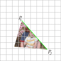
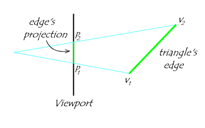
First, let's consider one edge from a given triangle. This edge and its projection onto our viewport lie in a single common plane. For the moment, let's look only at that plane, which is illustrated below: |
 |
 |
 |
 ,
, 
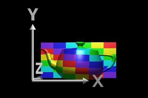
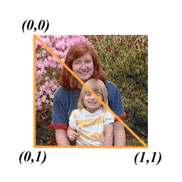
In two-dimensional texture mapping, we have to decide how to paste the image on to an object. In other words, for each pixel in an object, we encounter the question, "Where do I have to look in the texture map to find the color?" To answer this question, we consider two things: map shape and map entity.
We’ll discuss map shapes first. For a map shape that’s planar, we take an ( x,y,z ) value from the object and throw away (project) one of the components, which leaves us with a two-dimensional (planar) coordinate. We use the planar coordinate to look up the color in the texture map.
Source : Teaching Texture Mapping Visually by Rosalee Wolfe / DePaul University / wolfe@cs.depaul.edu
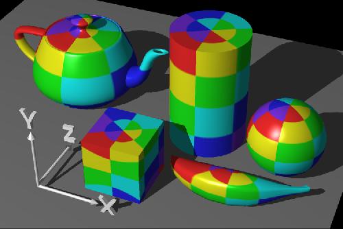
This slide shows several textured-mapped objects that have a planar map shape. None of the objects have been rotated. In this case, the component that was thrown away was the z-coordinate. You can determine which component was projected by looking for color changes in coordinate directions. When moving parallel to the x-axis, an object’s color changes. When moving up and down along the y-axis, the object’s color also changes. However, movement along the z-axis does not produce a change in color. This is how you can tell that the z-component was eliminated.
Source : Teaching Texture Mapping Visually by Rosalee Wolfe / DePaul University / wolfe@cs.depaul.edu
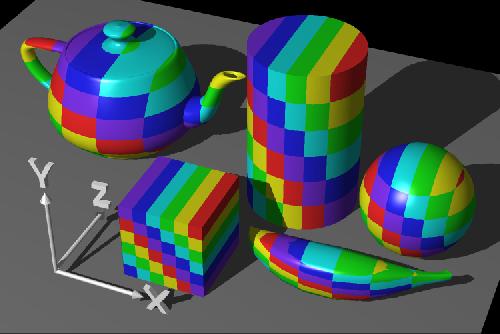
A second shape used in texture mapping is a cylinder. An ( x,y,z ) value is converted to cylindrical coordinates of ( r, theta, height ). For texture mapping, we are only interested in theta and the heigh t. To find the color in two-dimensional texture map, theta is converted into an x-coordinate and height is converted into a y-coordinate. This wraps the two-dimensional texture map around the object.
The texture-mapped objects in this image have a cylindrical map shape, and the cylinder’s axis is parallel to the z-axis. At the smallest z-position on each object, note that the squares of the texture pattern become squeezed into "pie slices". This phenomenon occurs at the greatest zposition as well. When the cylinder’s axis is parallel to the z-axis, you’ll see "pie slices" radiating out along the x- and y- axes.
Source : Teaching Texture Mapping Visually by Rosalee Wolfe / DePaul University / wolfe@cs.depaul.edu
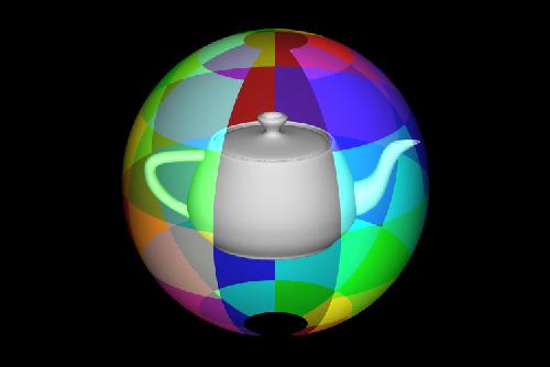
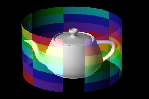
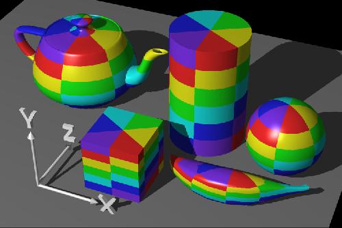
When using a sphere as the map shape, the ( x,y,z ) value of a point is converted into spherical coordinates. For purposes of texture mapping, we keep just the latitude and the longitude information. To find the color in the texture map, the latitude is converted into an x-coordinate and the longitude is converted into a y-coordinate.
The objects have a map shape of a sphere, and the poles of the sphere are parallel to the y-axis. At the object’s "North Pole" and "South Pole", the squares of the texture map become squeezed into pie-wedge shapes. Compare this to a map shape of a cylinder. Both map shapes have the pie-wedge shapes at the poles, but there is a subtle difference at the object’s "equator". The spherical mapping stretches the squares in the texture map near the equator, and squeezes the squares as the longitude reaches a pole.
Source : Teaching Texture Mapping Visually by Rosalee Wolfe / DePaul University / wolfe@cs.depaul.edu
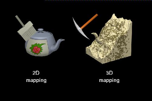
Texture mapping can be divided into two-dimensional and three-dimensional techniques. Two-dimensional techniques place a two-dimensional (flat) image onto an object using methods similar to pasting wallpaper onto an object. Three-dimensional techniques are analogous to carving the object from a block of marble.
In three-dimensional texture mapping, each point determines its color without the use of an intermediate map shape (Peachey, 1985; Perlin, 1985). We use the (x,y,z) coordinate to compute the color directly. It’s equivalent to carving an object out of a solid substance.
Most 3D texture functions do not explicitly store a value for each (x, y, z)-coordinate, but use a procedure to compute a value based on the coordinate and thus are called procedural textures.
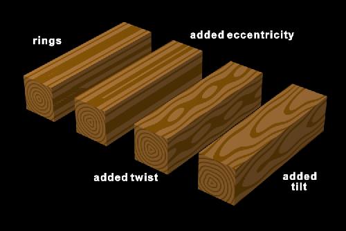
Perturbing stripes can result in a texture with a marbled appearance.
Making a wood-grained object begins with a three-dimensional texture of concentric rings (Peachey, 1985). By using noise to vary the ring shape and the inter-ring distance, we can create reasonably realistic wood.
We detect bumps in a surface by the relative darkness or lightness of the surface feature. In local illumination models, this is primarily determined by the direct diffuse reflection term which is proportional to N*L. N is the surface normal and L is the light vector. By modifying N, we can create spots of darkness or brightness.
James Blinn invented the method of perturbing the surface normal, N, by a "wrinkle" function. This changes the light interaction but not the actual size of the objects so that bump mapped objects appear smooth at the silhouette.
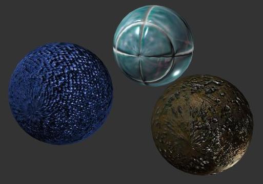
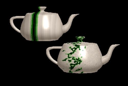
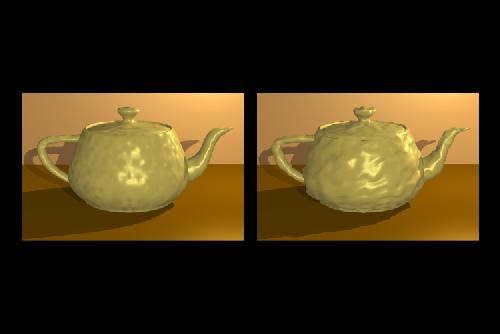
Here is an example of bump mapping. Notice that for both this image and the one below that the surfaces appear to have bumps or gouges but that the silhouette of the object is still smooth.
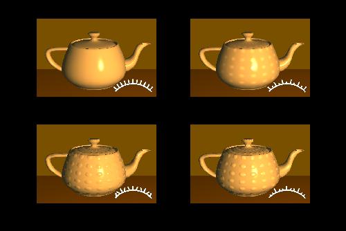
Bump mapping affects object surfaces, making them appear rough, wrinkled, or dented (Blinn, 1978). Bump mapping alters the surface normals before the shading calculation takes place. It’s possible to change a surface normals magnitude or direction.
In displacement mapping, the surface is actually modified, in contrast to bump mapping where only the surface normal is modified. This means that displacement mapped surfaces will show the effect even at the silhouette.
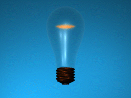
A Pixar Renderman image with displacement mapping. Notice that the surface not only appears non-smooth but the silhouette is also non-smooth.
In contast, displacement mapping alters an object’s geometry (Cook, 1984). Compare the profiles and the shadows cast by these two objects. Which is bump mapped?
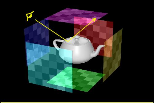
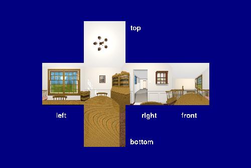
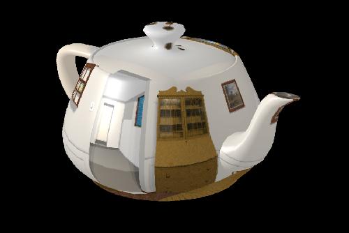
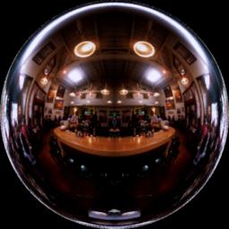
Environment mapping is a cheap way to create reflections (Blinn and Newell, 1976). While it’s easy to create reflections with a ray tracer, ray tracing is still too expensive for long animations. Adding an environment mapping feature to a z-buffer based renderer will create reflections that are acceptable in a lot of situations. Environment mapping is a two-dimensional texture mapping technique that uses a map shape of a box and a map parameter of a reflection ray.
a la SGI ClearCoat.
Lightscape / VRML