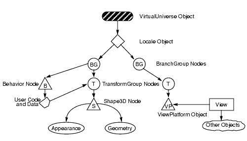
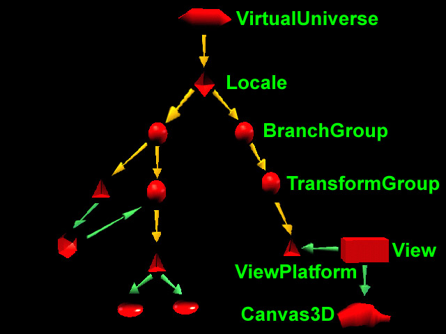
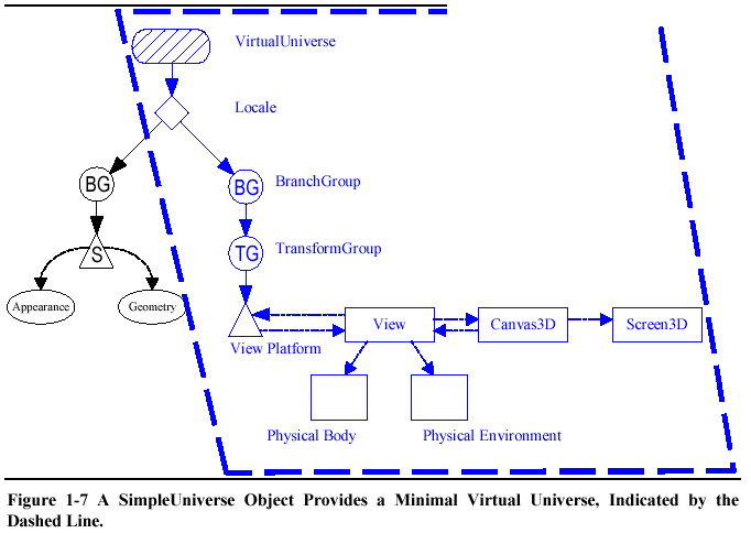
	//	This is the root of our view branch
viewBranch = new BranchGroup();

	//	The transform that will move our view
viewTransform = new Transform3D();
viewTransform.set(new Vector3f(0.0f,0.0f,5.0f));

	//	The transform group that will be the parent
	//	of our view platform elements
viewTransformGroup = new TransformGroup(viewTransform);
viewTransformGroup.setCapability(TransformGroup.ALLOW_TRANSFORM_WRITE);
myViewPlatform = new ViewPlatform();

	//	Next the physical elements are created
myBody = new PhysicalBody();
myEnvironment = new PhysicalEnvironment();

	//	Then we put it all together
viewTransformGroup.addChild(myViewPlatform);
viewBranch.addChild(viewTransformGroup);
myView = new View();
myView.addCanvas3D(this);
myView.attachViewPlatform(myViewPlatform);
myView.setPhysicalBody(myBody);
myView.setPhysicalEnvironment(myEnvironment);

	//	Create a default universe and locale
myUniverse = new VirtualUniverse();
myLocale = new Locale(myUniverse);

	// Create the content Branch
contentBranch = new BranchGroup();
contentTransform = new Transform3D();
contentTransform.set(new AxisAngle4d(1.0,1.0,0.0,Math.PI/4.0));
contentTransformGroup = new TransformGroup(contentTransform);
contentBranch.addChild(contentTransformGroup);
	// buildShape and addLights are two personal methos to implement to
	// get some result.
contentTransformGroup.addChild(buildShape());
addLights(contentBranch);

	//Use the functions to build the scene graph
myLocale.addBranchGraph(viewBranch);
myLocale.addBranchGraph(contentBranch);
/**
 *  This program demonstrate a very simple way to use the Wedge API : Tiwi
 */

import javax.media.j3d.*;
import com.sun.j3d.utils.geometry.Sphere;
import com.sun.j3d.utils.geometry.Cylinder;
import javax.vecmath.*;
import java.awt.*;


import escience.tiwi.*;
import escience.util.virtracker.*;
import escience.util.controls.KeyControls;


public class SimpleWedge  {


        /**     In order to move a virtual head in front of the screen if you are not
using the wedge
        real Head Tracker       */
        private Virtracker      vt;
        private Wedge           wedge;
;

        /**   the configuration class  */
        public SimpleWedge() {

                // setup configuration 1 : ask for what you would like
                WedgeConfigTemplate template = new WedgeConfigTemplate();

                template.setStereo(WedgeConfigTemplate.PREFERRED);
                template.setNumWalls(2);
                template.setHeadTracking(WedgeConfigTemplate.PREFERRED);
                template.setVirTracking(WedgeConfigTemplate.REQUIRED);
                template.setDisplayFrameRate(WedgeConfigTemplate.PREFERRED);

                // set up configuration 2 : Here is what you could get
                WedgeConfiguration config = new WedgeConfiguration(template);

                // Create our own wedge for the view with a class method
                // there should be only one !
                wedge = Wedge.getWedge(config);

                // Head Virtual Tracker
                vt = wedge.getVT();
                if (vt == null) {
                        System.out.println("Error: no Virtracker device");
                }

                Canvas3D leftCanvas = wedge.getCanvas(wedge.LEFT_WALL);
                if (leftCanvas != null)
                        leftCanvas.addKeyListener( new KeyHandler(vt) );
                else
                        System.out.println("Error: should have at least one canvas");
                Canvas3D rightCanvas = wedge.getCanvas(wedge.RIGHT_WALL);
                if (rightCanvas != null)
                        rightCanvas.addKeyListener( new KeyHandler(vt) );


                // Content creation
                IterText points = new IterText();

                // create an arbitrary application scene graph and view branch
                // to place the viewPlatform

                BranchGroup scene = points.createSceneGraph();

                // add a content Branch to your wedge object
                wedge.addBranchGraph(scene);

        }

        public static void main(String[] args) {

                SimpleWedge simple = new SimpleWedge();
        }
}


/**
 * This class contains a method to create a scenegraph of points in
 * virtual space.  Points one meter apart are red spheres, and intermediate
 * points are yellow. SharedGroups and links are used to minimise the number
 * of objects in the scene graph.
 */
 class IterText {

    private static final int numX = 5;
    private static final int numY = 3;
    private static final int numZ = 5;
    private static final int offsetX = -2;
    private static final int offsetY = 0;
    private static final int offsetZ = -2;

    private String fontName = "TestFont";
    private double tessellation = 0.0;

    private Color3f red       = new Color3f(1.0f, 0.0f, 0.0f);
    private Color3f green     = new Color3f(0.0f, 1.0f, 0.0f);
    private Color3f blue      = new Color3f(0.0f, 0.0f, 1.0f);
    private Color3f yellow    = new Color3f(1.0f, 1.0f, 0.0f);
    private Color3f black     = new Color3f(0.0f, 0.0f, 0.0f);
    private Color3f white     = new Color3f(1.0f, 1.0f, 1.0f);
    private Color3f lColor2   = new Color3f(0.0f, 1.0f, 0.0f);
    private Color3f alColor   = new Color3f(0.2f, 0.2f, 0.2f);
    private Color3f bgColor  = new Color3f(0.05f, 0.05f, 0.2f);

    private Shape3D display = null;
    private Font3D f3d = new Font3D(new Font(fontName, Font.PLAIN, 2),
                            new FontExtrusion());

    public IterText() {};

    /**
     * This method creates the scene graph as described above.
     */
    public BranchGroup createSceneGraph() {

        int posX, posY, posZ;

        Appearance whiteA = new Appearance();
        Material whiteM = new Material();
        whiteM.setLightingEnable(true);
        whiteM.setEmissiveColor(white);
        whiteA.setMaterial(whiteM);

        Appearance redA = new Appearance();
        Material redM = new Material();
        redM.setLightingEnable(true);
        redM.setEmissiveColor(red);
        redA.setMaterial(redM);

        Appearance yellowA = new Appearance();
        Material yellowM = new Material();
        yellowM.setLightingEnable(true);
        yellowM.setEmissiveColor(yellow);
        yellowA.setMaterial(yellowM);


        // objects for one meter coordinates
        TransformGroup[][][] tg = new TransformGroup[numX][numY][numZ];
        Transform3D[][][] t3d = new Transform3D[numX][numY][numZ];
        Link[][][] link = new Link[numX][numY][numZ];
        Sphere redSp = new Sphere(0.5f, Sphere.GENERATE_NORMALS, 10, redA);
        Shape3D[][][] sh = new Shape3D[numX][numY][numZ];

        // objects for intermediate coodinates
        TransformGroup[][][] itgy = new TransformGroup[numX][numY][numZ];
        Transform3D[][][] it3dy = new Transform3D[numX][numY][numZ];
        Link[][][] iLinky = new Link[numX][numY][numZ];
        TransformGroup[][][] itgz = new TransformGroup[numX][numY][numZ];
        Transform3D[][][] it3dz = new Transform3D[numX][numY][numZ];
        Link[][][] iLinkz = new Link[numX][numY][numZ];
        Sphere yellowSp = new Sphere(0.5f, Sphere.GENERATE_NORMALS, 10, yellowA);

        // Shared Group Nodes
        SharedGroup redSG = new SharedGroup();
        redSG.addChild(redSp);
        redSG.compile();
        SharedGroup yellowSG = new SharedGroup();
        yellowSG.addChild(yellowSp);
        yellowSG.compile();

        // Create the root of the branch graph
        BranchGroup objRoot = new BranchGroup();

        objRoot.setCapability(objRoot.ALLOW_CHILDREN_WRITE);
        // Create the transform group node and initialize it to the
        // identity.  Enable the TRANSFORM_WRITE capability so that
        // our behavior code can modify it at runtime.  Add it to the
        // root of the subgraph.

        // draw cylinders for xyz axis
        // first y axis
        TransformGroup yAxisTG = new TransformGroup();
        Transform3D atY = new Transform3D();
        atY.setTranslation(new Vector3d(0.0, 0.0, 0.0));
        yAxisTG.setTransform(atY);
        yAxisTG.setCapability(TransformGroup.ALLOW_TRANSFORM_WRITE);
        objRoot.addChild(yAxisTG);

        Material axisMatY = new Material(black, green, black, black, 100.0f);
        Appearance axisAppY = new Appearance();
        axisMatY.setLightingEnable(true);
        axisAppY.setMaterial(axisMatY);
        Cylinder yAxis = new Cylinder(0.01f, 5.0f, Cylinder.GENERATE_NORMALS,
axisAppY);
        yAxisTG.addChild(yAxis);
        // then x Axis
        TransformGroup xAxisTG = new TransformGroup();
        Transform3D atX = new Transform3D();
        atX.setTranslation(new Vector3d(0.0, 0.0, 0.0));
        atX.rotZ(Math.toRadians(90));
        xAxisTG.setTransform(atX);
        xAxisTG.setCapability(TransformGroup.ALLOW_TRANSFORM_WRITE);
        objRoot.addChild(xAxisTG);

        Material axisMatX = new Material(black, red, black, black, 100.0f);
        Appearance axisAppX = new Appearance();
        axisMatX.setLightingEnable(true);
        axisAppX.setMaterial(axisMatX);
        Cylinder xAxis = new Cylinder(0.01f, 5.0f, Cylinder.GENERATE_NORMALS,
axisAppX);
        xAxisTG.addChild(xAxis);
        // then z axis
        TransformGroup zAxisTG = new TransformGroup();
        Transform3D atZ = new Transform3D();
        atZ.setTranslation(new Vector3d(0.0, 0.0, 0.0));
        atZ.rotX(Math.toRadians(90));
        zAxisTG.setTransform(atZ);
        zAxisTG.setCapability(TransformGroup.ALLOW_TRANSFORM_WRITE);
        objRoot.addChild(zAxisTG);

        Material axisMatZ = new Material(black, blue, black, black, 100.0f);
        Appearance axisAppZ = new Appearance();
        axisMatZ.setLightingEnable(true);
        axisAppZ.setMaterial(axisMatZ);
        Cylinder zAxis = new Cylinder(0.01f, 5.0f, Cylinder.GENERATE_NORMALS,
axisAppZ);
        zAxisTG.addChild(zAxis);

        for (int x = 0; x < numX; x++) {
            for (int y = 0; y < numY; y++) {
                for (int z = 0; z < numZ; z++) {
                    posX = x + offsetX;
                    posY = y + offsetY;
                    posZ = z + offsetZ;

                    // place one meter coordinates, with text
                    tg[x][y][z] = new TransformGroup();
                    t3d[x][y][z] = new Transform3D();
                    t3d[x][y][z].setTranslation(new Vector3d(posX, posY, posZ));
                    t3d[x][y][z].setScale(0.04);
                    tg[x][y][z].setTransform(t3d[x][y][z]);
                    tg[x][y][z].setCapability(TransformGroup.ALLOW_TRANSFORM_WRITE);
                    link[x][y][z] = new Link(redSG);
                    objRoot.addChild(tg[x][y][z]);

                    String str = new String("(" + posX + ", " + posY + ", " + posZ + ")");
                    Text3D txt = new Text3D(f3d, str,
                                            new Point3f(0.001f, 0.0f, 0.0f));
                    sh[x][y][z] = new Shape3D();
                    sh[x][y][z].setAppearance(whiteA);
                    sh[x][y][z].setGeometry(txt);

                    tg[x][y][z].addChild(sh[x][y][z]);
                    tg[x][y][z].addChild(link[x][y][z]);

                    // now do intermediates
                    // first posY + a half meter
                    itgy[x][y][z] = new TransformGroup();
                    it3dy[x][y][z] = new Transform3D();
                    it3dy[x][y][z].setTranslation(new Vector3d(posX, posY + 0.5, posZ));
                    it3dy[x][y][z].setScale(0.02);
                    itgy[x][y][z].setTransform(it3dy[x][y][z]);
                    itgy[x][y][z].setCapability(TransformGroup.ALLOW_TRANSFORM_WRITE);
                    iLinky[x][y][z] = new Link(yellowSG);
                    objRoot.addChild(itgy[x][y][z]);

                    itgy[x][y][z].addChild(iLinky[x][y][z]);

                    // then posZ + a half meter
                    itgz[x][y][z] = new TransformGroup();
                    it3dz[x][y][z] = new Transform3D();
                    it3dz[x][y][z].setTranslation(new Vector3d(posX, posY, posZ + 0.5));
                    it3dz[x][y][z].setScale(0.02);
                    itgz[x][y][z].setTransform(it3dz[x][y][z]);
                    itgz[x][y][z].setCapability(TransformGroup.ALLOW_TRANSFORM_WRITE);
                    iLinkz[x][y][z] = new Link(yellowSG);
                    objRoot.addChild(itgz[x][y][z]);

                    //ispz[x][y][z] = new Sphere(0.5f, Sphere.GENERATE_NORMALS, 10,
ia[x][y][z]);
                    itgz[x][y][z].addChild(iLinkz[x][y][z]);

                }
            }
        }


        // Have Java 3D perform optimizations on this scene graph.
        objRoot.compile();

        return objRoot;
    }
}
A CRT is an evacuated glass tube, with a heating element on one end and a phosphor coated screen on the other
Rasterisation = Pixelisation
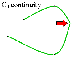
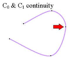
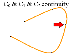
|
Zero order parametric continuityThe curves meet |
First order parametric continuitythe tangents are shared |
Second order parametric continuitythe"speed" is the same before and afteranimation paths... |
Some of theses properties may sound somewhere obvious, but they are presented here because they are still valid for Bézier curves of higher degree
The degree of the polynomial is always one less than the number of control points. In computer graphics, we generally use degree 3. Quadratic curves are not flexible enough and going above degree 3 gives rises to complications and so the choice of cubics is the best compromise for most computer graphics applications.
Moving any control point affects all of the curve to a greater or lesser extent. All the basis functions are everywhere non-zero except at the point u = 0 and u = 1
This is the basis of the intuitive 'feel' of a Bézier curve interface.
The curve does not oscillate about any straight line more often than the control point polygon
The curve is transformed by applying any affine transformation (that is, any combination of linear transformations) to its control point representation. The curve is invariant (does not change shape) under such a transformation.
As soon as you move one control point, you affect the entire curve
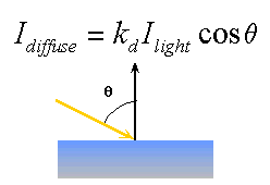
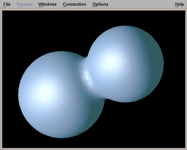
Java3D : Real Time illumination model : lots of approximations. No Shade, simplified transparency, no reflexion (miror).
Raytracing, Radiosity...
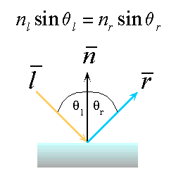 Reflection : a special case of the Snell / Descartes law
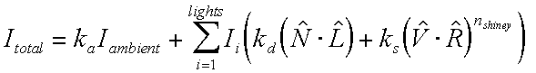
1. Application/Scene
2. Geometry
3. Triangle Setup
4. Rendering / Rasterization
|
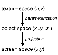
Objects in the 3D scene and the scene itself are sequentially converted, or
transformed, through five spaces when proceeding through the 3D pipeline. A
brief overview of these spaces follows:
where each model is in its own coordinate system, whose origin is some point on the model, such as the right foot of a soccer player model. Also, the model will typically have a control point or "handle". To move the model, the 3D renderer only has to move the control point, because model space coordinates of the object remain constant relative to its control point. Additionally, by using that same "handle", the object can be rotated.
where models are placed in the actual 3D world, in a unified world coordinate system. It turns out that many 3D programs skip past world space and instead go directly to clip or view space. The OpenGL API doesn't really have a world space.
in this space, the view camera is positioned by the application
(through the graphics API) at some point in the 3D world coordinate system,
if it is being used. The world space coordinate system is then transformed,
such that the camera (your eye point) is now at the origin of the coordinate
system, looking straight down the z-axis into the scene. If world space is bypassed,
then the scene is transformed directly into view space, with the camera similarly
placed at the origin and looking straight down the z-axis. Whether z values
are increasing or decreasing as you move forward away from the camera into the
scene is up to the programmer, but for now assume that z values are increasing
as you look into the scene down the z-axis. Note that culling, back-face culling,
and lighting operations can be done in view space.
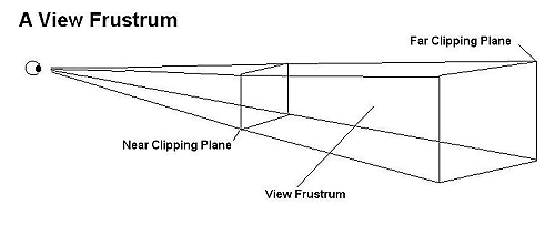
The view volume is actually created by a projection, which as the name suggests,
"projects the scene" in front of the camera. In this sense, it's a
kind of role reversal in that the camera now becomes a projector, and the scene's
view volume is defined in relation to the camera. Think of the camera as a kind
of holographic projector, but instead of projecting a 3D image into air, it
instead projects the 3D scene "into" your monitor. The shape of this
view volume is either rectangular (called a parallel projection), or
pyramidal (called a perspective projection), and this latter volume is
called a view frustum (also commonly called frustrum, though frustum
is the more current designation).
The view volume defines what the camera will see, but just as importantly, it
defines what the camera won't see, and in so doing, many objects models and
parts of the world can be discarded, sparing both 3D chip cycles and memory
bandwidth.
The frustum actually looks like an pyramid with its top cut off. The top of
the inverted pyramid projection is closest to the camera's viewpoint and radiates
outward. The top of the frustum is called the near (or front) clipping
plane and the back is called the far (or back) clipping plane. The entire
rendered 3D scene must fit between the near and far clipping planes, and also
be bounded by the sides and top of the frustum. If triangles of the model (or
parts of the world space) falls outside the frustum, they won't be processed.
Similarly, if a triangle is partly inside and partly outside the frustrum the
external portion will be clipped off at the frustum boundary, and thus the term
clipping. Though the view space frustum has clipping planes, clipping
is actually performed when the frustum is transformed to clip space.
Similar to View Space, but the frustum is now "squished" into a unit cube, with the x and y coordinates normalized to a range between –1 and 1, and z is between 0 and 1, which simplifies clipping calculations. The "perspective divide" performs the normalization feat, by dividing all x, y, and z vertex coordinates by a special "w" value, which is a scaling factor that we'll soon discuss in more detail. The perspective divide makes nearer objects larger, and farther objects smaller as you would expect when viewing a scene in reality.
where the 3D image is converted into x and y 2D screen coordinates for 2D display. Note that z and w coordinates are still retained by the graphics systems for depth/Z-buffering (see Z-buffering section below) and back-face culling before the final render. Note that the conversion of the scene to pixels, called rasterization, has not yet occurred.
Because so many of the conversions involved in transforming through these different
spaces essentially are changing the frame of reference, it's easy to get confused.
Part of what makes the 3D pipeline confusing is that there isn't one "definitive"
way to perform all of these operations, since researchers and programmers have
discovered different tricks and optimizations that work for them, and because
there are often multiple viable ways to solve a given 3D/mathematical problem.
But, in general, the space conversion process follows the order we just described.
To get an idea about how these different spaces interact, consider this example:
Take several pieces of Lego, and snap them together to make some object. Think
of the individual pieces of Lego as the object's edges, with vertices existing
where the Legos interconnect (while Lego construction does not form triangles,
the most popular primitive in 3D modeling, but rather quadrilaterals, our example
will still work). Placing the object in front of you, the origin of the model
space coordinates could be the lower left near corner of the object, and all
other model coordinates would be measured from there. The origin can actually
be any part of the model, but the lower left near corner is often used. As you
move this object around a room (the 3D world space or view space, depending
on the 3D system), the Lego pieces' positions relative to one another remain
constant (model space), although their coordinates change in relation to the
room (world or view spaces). In some sense, 3D chips have become physical incarnations
of the pipeline, where data flows "downstream" from stage to stage.
It is useful to note that most operations in the application/scene stage and
the early geometry stage of the pipeline are done per vertex, whereas culling
and clipping is done per triangle, and rendering operations are done per pixel.
Computations in various stages of the pipeline can be overlapped, for improved
performance. For example, because vertices and pixels are mutually independent
of one another in both Direct3D and OpenGL, one triangle can be in the geometry
stage while another is in the Rasterization stage. Furthermore, computations
on two or more vertices in the Geometry stage and two or more pixels (from the
same triangle) in the Rasterzation phase can be performed at the same time.
Another advantage of pipelining is that because no data is passed from one vertex
to another in the geometry stage or from one pixel to another in the rendering
stage, chipmakers have been able to implement multiple pixel pipes and gain
considerable performance boosts using parallel processing of these independent
entities. It's also useful to note that the use of pipelining for real-time
rendering, though it has many advantages, is not without downsides. For instance,
once a triangle is sent down the pipeline, the programmer has pretty much waved
goodbye to it. To get status or color/alpha information about that vertex once
it's in the pipe is very expensive in terms of performance, and can cause pipeline
stalls, a definite no-no.
ExtremeTech 3D Pipeline Tutorial
June, 2001
By: Dave Salvator
extract from http://www.extremetech.com/
geometry database gather necessary object information (the geometry database includes all the geometric primitives of the objects)
a visibility test that determines whether an object is partially or completely occluded (covered) by some object in front of it.
on each object. This can be accomplished by determining if the object is in the view frustum (completely or partially).
The original Quake used what were called potentially visible sets (PVS) that divided the world into smaller pieces. Essentially, if the game player was in a particular piece of the world, other areas would not be visible, and the game engine wouldn't have to process data for those parts of the world.
Check the bounding box intead of the object
The distance from the object to the view camera will dictate which LOD level gets used.
because connected triangles share vertices...
These are curved primitives that have more complex mathematical descriptions, but in some cases, this added complexity is still cheaper than describing an object with a multitude of triangles. These primitives have some pretty odd sounding names: parametric polynomials (called SPLINEs), non-uniform rational b-splines (NURBs), Beziers, parametric bicubic surfaces and n-patches.
The first step in reducing the working set of triangles to be processed is to cull ("select from a group") those that are completely outside of the view volume as we noted previously. This process is called "trivial rejection," because relative to clipping, this is a fairly simple operation.
A test is performed to determine if the x, y, and z coordinates of a triangle's three vertices are completely outside of the view volume (frustum). In addition, the triangle's three vertices have to be completely outside the view volume on the same side of the view frustum, otherwise it could possible for a part of the triangle to pass through the view frustum, even though its three vertices lie completely outside the frustum.
if (primitive isn't trivially rejected)
	and if (primitive is trivially accepted)
		draw it
else
   clip it and draw that part of the triangle that's inside the view volume
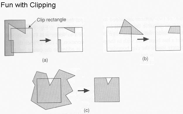
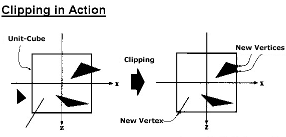
Taking Sutherland-Hodgeman as an example, this algorithm can work in either 2D (four clipping boundaries) or in 3D (six clipping boundaries--left, right, top, bottom, near, far). It works by examining a triangle one boundary at a time, and in some sense is a "multi-pass" algorithm, in that it initially clips against the first clip boundary. It then takes the newly clipped polygon and compares it to the next clip boundary, re-clips if necessary, and ultimately does six "passes" in order to clip a triangle against the six sides of the 3D unit cube.
Once a triangle has been clipped, it must be retesselated, or made into a new set of triangles. Take for example the diagram where you see a single triangle being clipped whose remaining visible portion now forms a quadrilateral. The clipper must now determine the intersection points of each side of the triangle with that clipping boundary, and then draws new triangles that will be part of the final scene.
Rendering is the series of operations that determine the final pixel colour displayed for a frame of animation, and while this can be thought of broadly as rasterization, the actual conversion of the 3D scene into screen-addressed pixels, or "real" rasterization, happens during triangle setup, also called scan-line conversion.
In the case of graphics cards (or printers), this process turns an image into points of colour. A rasterizer can be a 3D card, or it can be a printer for that matter
Aliasing is a potential problem whenever an analog signal is point sampled to convert it into a digital signal. It can occur in audio sampling, for example, in converting music to digital form to be stored on a CD-ROM or other digital device. Aliasing happens whenever an analog signal is not sampled at a high enough frequency. In audio, Aliasing manifests itself in the form of spurious low frequencies. An example is shown below of two sin waves.
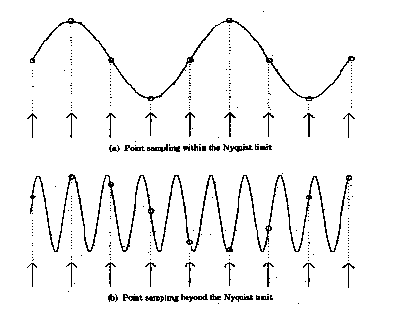
Image Reference : Robert L. Cook, "Stochastic Sampling and Distributed Ray Tracing", An Introduction to Ray Tracing, Andrew Glassner, ed., Academic Press Limited, 1989.
In the top sin wave, the sampling is fast enough that a reconstructed signal (the small circles) would have the same frequency as the original sin wave. In the bottom wave, with a higher frequency but the same point sampling rate, a reconstructed signal (the small circles) would appear to be a sin wave of a lower frequency, i.e., an aliased signal.
From Point Sampling Theory it turns out that to accurately reconstruct a signal, the signal must be sampled at a rate greater than or equal to two times the highest frequency contained in the signal. This is called the Nyquist Theorem and the highest frequency that can be accurately represented with a given sampling rate is called the Nyquist limit. For example, to produce a music CD-ROM the analog signal is sampled at a maximum rate of 44 Khz, therefore the highest possible audio frequency is 22khz. Any audio frequencies greater than 22Khz must be removed from the input signal or they will be aliased, i.e., appear as low frequency sounds.
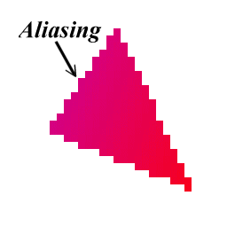
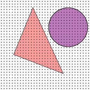
Aliasing occurs in computer graphics, since we are point sampling an analog signal. The mathematical model of an image is a continuous analog signal which is sampled at discrete points (the pixel positions). When the sampling rate is less than Nyquist Limit then there are aliasing artifacts that are called "jaggies" in computer graphics. In general, aliasing is when high frequencies appear as low frequencies which produce regular patterns easy to see.
When a continuous image is multiplied by a sampling grid a discrete set of points are generated. These points are called samples. These samples are pixels. We store them in memory as arrays of numbers representing the intensity of the underlying function.
In order to have any hope of accurately reconstructing a function from a periodically sampled version of it, two conditions must be satisfied:
In practice:
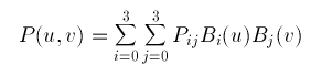
If one parameter is held at a constant value then the above will represent
a curve. Thus P(u,a) is a curve on the surface with the parameter v being a
constant a.
In a bicubic surface patch cubic polynomials are used to represent the edge
curves P(u,0), P(u,1), P(0,v) and P(1,v)as shown below. The surface is then
generated by sweeping all points on the boundary curve P(u,0) (say) through
cubic trajectories,defined using the parameter v, to the boundary curve P(u,1).
In this process the role of the parameters u and v can be reversed.
![]()
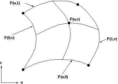
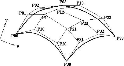
The representation of the bicubic surface patch can be
illustrated by considering the Bezier Surface Patch.
The edge P(0,v) of a Bezier patch is defined by giving four control points P00,
P01, P02 and P03. Similarly the opposite edge P(1,v) can be represented by a
Bezier curve with four control points. The surface patch is generated by sweeping
the curve P(0,v) through a cubic trajectory in the parameter u to P(1,v). To
define this trajectory we need four control points, hence the Bezier surface
patch requires a mesh of 4*4 control points as illustrated below.
The method of Constructive Solid Geometry arose from the observation that many industrial components derive from combinations of various simple geometric shapes such as spheres, cones, cylinders and rectangular solids. In fact the whole design process often started with a simple block which might have simple shapes cut out of it, perhaps other shapes added on etc. in producing the final design. For example consider the simple solid below:
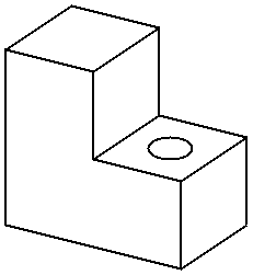
This simple component could be produced by gluing two rectangular blocks together and then drilling the hole. Or in CSG terms the the union of two blocks would be taken and then the difference of the resultant solid and a cylinder would be taken. In carrying out these operations the basic primitive objects, the blocks and the cylinder, would have to be scaled to the correct size, possibly oriented and then placed in the correct relative positions to each other before carrying out the logical operations.
The Boolean Set Operators used are:
Note that the above definitions are not rigorous and have to be refined to define the Regularised Boolean Set Operations to avoid impossible solids being generated.
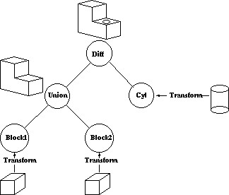
A CSG model is then held as a tree structure whose terminal nodes are primitive objects together with an appropriate transformation and whose other nodes are Boolean Set Operations. This is illustrated below for the object above which is constructed using cube and cylinder primitives.
CSG methods are useful both as a method of representation and as a user interface technique. A user can be supplied with a set of primitive solids and can combine them interactively using the boolean set operators to produce more complex objects. Editing a CSG representation is also easy, for example changing the diameter of the hole in the example above is merely a case of changing the diameter of the cylinder.
However it is slow to produce a rendered image of a model from a CSG tree. This is because most rendering pipelines work on B-reps and the CSG representation has to be converted to this form before rendering. Hence some solid modellers use a B-rep but the user interface is based on the CSG representation.
http://www.forums.pctechguide.com/glossary/bycat.php?catSelected=6&catSearchSubmit=View+Category
"Still" graphic terms explained (not multimedia)
| Term | Definition |
|---|---|
| 3D API | A 3D application programming interface controls all aspects of the 3D rendering process. A mass of conflicting standards exist, including Microsoft’s DirectX and OpenGL, Intel’s 3DR, Reality Lab and Brender. Most are custom designed for either entertainment or serious 3D animation. |
| 3D Graphics | The display of objects and scenes with height, width, and depth information. The information is calculated in a co-ordinate system that represents three dimensions via x, y, and z axes. |
| Addressability | Refers to how many pixels can be sent to the display horizontally and vertically. The most common combinations currently in use are 640x480 (VGA mode), 800x600 (SVGA mode), 1024x768, 1280x1024 and 1600x1200. |
| Aliasing | A form of image distortion associated with signal sampling. A common form of aliasing is a stair-stepped appearance along diagonal and curved lines. |
| Alpha | Additional colour component in some representations of pixels, along with red, green, and blue (RGB). The alpha channel denotes transparency or opacity, often as a fractional value, used in blending and anti-aliasing. |
| Alpha Blending | An approach which uses the alpha channel to control how an object or bitmap interacts visually with its surroundings. It can be used to layer multiple textures onto a 3D object, or to simulate the translucency of glass or mask out areas of background. |
| Alpha Channel | The extra layer of 8-bit greyscale carried by a 32-bit graphic. This extra information is used to determine the transparency or edge characteristics of the image. |
| Anamorphic | Unequally scaled in vertical and horizontal dimensions. |
| Anti-aliasing | Hides the jagged effect of image diagonals (sometimes called jaggies) by modulating the intensity on either side of the diagonal boundaries, creating localised blurring along these edges and reducing the appearance of stepping. |
| Artefact | Unsightly visual side effect caused by defects in compression or other digital manipulation. Common artefacts include jaggies, polygon shearing (where 3D objects are torn or warped when screen refreshes can't keep up with 3D activity) and pixelation (where texture maps lose resolution and look blocky close up). |
| Asymmetrical Compression | A system which requires more processing capability to compress an image than to decompress an image. It is typically used for the mass distribution of programs on media such as CD-ROM, where significant expense can be incurred for the production and compression of the program but the playback system must be low in cost. |
| Back Buffer | A hidden drawing buffer used in double-buffering. Graphics are drawn into the back buffer so that the rendering process cannot be seen by the user. When the drawing is complete, the front and back buffers are swapped. |
| Bezier | A way of mathematically describing a curve, used by graphics programs such as MacroMedia FreeHand and Adobe Illustrator. |
| Bi-linear Filtering | Improves the look of blocky, low-resolution 3D textures when viewed close up by blending and interpolating groups of texels to create a smoother image. |
| Bit Depth | In colour images, the number of colours used to represent the image. Typical values are 8-, 16-, and 24-bit colour, allowing 256, 65,536 and 16,777,216 colours to be represented. The latter is known as true colour, because 16.8 million different colours is about as many as the human eye can distinguish. Also referred to as colour depth. |
| Bitmap File | File in which every pixel on screen is represented by a piece of data in memory, usually graphics although some audio formats are described as bitmapped as well. As opposed to a vector image, in which only a description of the image is stored. Each pixel can be represented by one bit (simple black and white) or up to 32 bits (high-definition colour). Uses the file extension "BMP". |
| Blockiness | The consequence of portions of an image breaking into little squares due to over-compression or a video file overwhelming a computer’s processor. See also Artefact. |
| BLT | Bit-aLigned BLock Transfer: the process of copying pixels or other data from one place in memory to another. |
| BPP | Bits Per Pixel: the number of bits used to represent the colour value of each pixel in a digitised image. |
| Brightness | A measure of the overall intensity of the image. The lower the brightness value, the darker the image; the higher the value, the lighter the image will be. |
| Bump Mapping | A 3D rendering lighting technique designed to give a texture a three-dimensional, animated feel. |
| Camera | In 3D graphics, the viewpoint through which a scene is viewed. Flythroughs of scenes are conceptually a moving camera. |
| CGA | Colour Graphics Adapter: a low-resolution video display standard, invented for the first IBM PC. CGA's highest resolution mode is 2 colours at a resolution of 640 x 200 pixels. |
| Chroma | The colour portion of a video signal that includes hue and saturation information. Requires luminance, or light intensity, to make it visible. Also referred to as Chrominance. |
| CIE | Commission International de l'Eclairage: the international organisation that establishes methods for measuring colour. Their colour standards for colourmetric measurements are internationally accepted specifications that define colour values mathematically. |
| CIELAB (L*a*b*) | A colour model to approximate human vision. The model consists of three variables: L* for luminosity, a* for one colour axis, and b* for the other colour axis. CIELAB is a good model of the Munsell colour system and human vision. |
| CIELUV (L*u*v) | A colour space model produced in 1978 by the CIE at the same time as the L*a*b model. CIE L*u*v is used with colour monitors, whereas CIE L*a*b is used with colour print production. |
| Clip Art | A collection of icons, buttons and other useful image files, along with sound and video files, that can be inserted into documents. |
| Clipping | Removing, from the processing pipeline to spare unneeded work, complete objects and surfaces which are outside the field of view (known as the "viewing frustrum"). Also known as Culling. |
| CMYK | Cyan, Magenta, Yellow, Black: the four process colours that are used in four-colour printed reproduction. |
| Colour Balance | The process of matching the amplitudes of red, green and blue signals so the resulting mixture makes an accurate white colour. |
| Colour Palette | Also called a colour lookup table (CLUT), index map, or colour map, it is a commonly-used method for saving file space when creating colour images. Instead of each pixel containing its own RGB values, which would require 24 bits, each pixel holds an 8-bit value, which is an index number into the colour palette. The colour palette contains a 256-colour subset of the 16 million unique displayable colours. |
| Compound Document | A file that has more than one element (text, graphics, voice, video) mixed together. |
| Continuous Tone | An image that has all the values (0 to 100%) of grey (black and white) or colour in it. A photograph is a continuous tone image. |
| Contrast | The range between the lightest tones and the darkest tones in an image. The lower the number value, the more closely the shades will resemble each other. The higher the number, the more the shades will stand out from each other. |
| DAC | Digital-to-Analogue Converter: a device (usually a single chip) that converts digital data into analogue signals. Video adapters require DACs to convert digital data to analogue signals that the monitor can process. |
| DCT | Discrete Cosine Transform: used in the JPEG and MPEG image compression algorithms. Refers to the coding methodology used to reduce the number of bits for actual data compression. DCT transforms a block of pixel intensities into a block of frequency transform coefficients. The transform is then applied to new blocks until the entire image is transformed. |
| Decal | A texture that is placed specifically on one part of a 3D object. |
| Decal Alpha Texture Blending | Decal texture blending with the addition of alpha transparency. |
| Decal Texture Blending | A blend technique where the triangle colour at each vertex is strictly the colour of the texture. The triangle's colour doesn't alter the texture colour. |
| Density | The degree of darkness of an image. Also, percent of screen used in an image. |
| Depth Cueing | Used in conjunction with fogging, depth cueing is the adjustment of the hue and colour of objects in relation to their distance from the viewpoint. |
| DIB File Format | Device-Independent Bitmap Format: a common bitmap format for Windows applications. |
| Dithering | The process of intentionally mixing colours of adjacent pixels. Dithering is usually needed for 8-bit colour, and sometimes for 16-bit. It allows a limited colour set to approximate a broader range, by mixing groups of varying-colour pixels in a semi-random pattern. Without dithering, colour gradients like sky or sunset tend to show "banding" artefacts. |
| DXF | Drawing Exchange Format: the industry standard 3D data format. |
| EGA | Enhanced Graphics Adapter: the IBM standard for colour displays prior to the VGA standard. It specified a resolution of 640x350 with up to 256 colours and a 9-pin (DB-9) connector. |
| Extrusion | Taking a flat, 2-D object and adding a z plane to expand it into 3-D space. |
| Flat Shading | The simplest form of 3D shading which fills polygons with one colour. Processor overheads are negligible and 3D games will allow the graphics to be stripped down to flat shading to improve the frame rate. |
| Fogging | The alteration of the visibility or clarity of an object, depending on how far the object is from the camera. Usually implemented by adding a fixed colour (fog colour) to each pixel. Also known as Haze. |
| Fractals | Along with raster and vector graphics, a way of defining graphics in a computer. Fractal graphics translate the natural curves of an object into mathematical formulas, from which the image can later be constructed. |
| Frame Buffer | Display memory that temporarily stores (buffers) a full frame of picture data at one time.Frame buffers are composed of arrays of bit values that correspond to the display’s pixels. The number of bits per pixel in the frame buffer determines the complexity of images that can be displayed. |
| Gamma | A mathematical curve representing both the contrast and brightness of an image. Moving the curve in one direction will make the image both darker and decrease the contrast. Moving the curve the other direction will make the image both lighter and increase the contrast. |
| Gamma Correction | A form of tone mapping in which the shape of the tone map is a gamma. |
| Gamma Curve | A mathematical function that describes the non-linear tonal response of many printers and monitors. A tone map that has the shape of this its compensating function cancels the nonlinearities in printers and monitors. |
| Gamut | The range of colours that can be captured or represented by a device. When a colour is outside a device's gamut, the device represents that colour as some other colour. |
| GDI | Graphics Device Interface: the component of Windows that permits applications to draw on screens, printers, and other output devices. The GDI provides hundreds of convenient functions for drawing lines, circles, and polygons, rendering fonts, querying devices for their output capabilities, and more. |
| Geometry | The computation of the base properties for each point (vertex) of the triangles forming the objects in the 3D world. These properties include x-y-z co-ordinates, RGB values, alpha translucency, reflectivity and others. The geometry calculations involve transformation from 3D world co-ordinates into corresponding 2-D screen co-ordinates, clipping off any parts not visible on screen and lighting. |
| GIF | Graphics Interchange Format: an image used by CompuServe and other on-line formats. Limited to 256 colours but supports transparency without an alpha channel and animation. |
| Gouraud Shading | A method of hiding the boundaries between polygons by modulating the light intensity across each one in a polygon mesh. |
| Gradient | In graphics, having an area smoothly blend from one colour to another, or from black to white, or vice versa. |
| Graphics Card | An expansion card that interprets drawing instructions sent by the CPU, processes them via a dedicated graphics processor and writes the resulting frame data to the frame buffer. Also called video adapter (the term "graphics accelerator" is no longer in use). |
| Graphics Library | A tool set for application programmers, interfaced with an application programmer’s interface, or API. The graphics library usually includes a defined set of primitives and function calls that enable the programmer to bypass many low-level programming tasks. |
| Graphics Processor | The specialised processor at the heart of the graphics card. Modern chipsets can also integrate video processing, 3D polygon setup and texturing routines, and, in some cases, the RAMDAC. |
| Greyscale | Shades of grey that represent light and dark portions of an image. Colour images can also be converted to greyscale where the colours are represented by various shades of grey. |
| GUI | Graphical User Interface: a graphics-based user interface that incorporates icons, pull-down menus and a mouse. The GUI has become the standard way for users to interact with a computer. The first graphical user interface was designed by Xerox Corporation’s Palo Alto Research Centre in the 1970s, but it was not until the 1980s and the emergence of the Apple Macintosh that graphical user interfaces became popular. The three major GUIs in popular use today are Windows, Macintosh and Motif. |
| Halftone | An image type that simulates greyscale by varying the sizes of the dots. Highly coloured areas consist of large colour dots, while lighter areas consist of smaller dots. |
| High Colour | Graphics cards that can show 16-bit colour (up to 65,536 colours). |
| Highlight | The brightest part of an image. |
| HSB | Hue Saturation Brightness: with the HSB model, all colours can be defined by expressing their levels of hue (the pigment), saturation (the amount of pigment) and brightness (the amount of white included), in percentages. |
| Hue | The attribute of a visual sensation according to which an area appears to be similar to one of the perceived colours, red, yellow, green and blue, or a combination of two of them. Also referred to as tint. |
| Image | The computerised representation of a picture or graphic. |
| Image Resolution | The fineness or coarseness of an image as it was digitised, measured in Dots Per Inch (DPI), typically from 200 to 400 DPI. |
| Interpolation | The process of averaging pixel information when scaling an image. When the size of an image is reduced, pixels are averaged to create a single new pixel; when an image is scaled up in size, additional pixels are created by averaging pixels of the smaller image. |
| Jaggies | Also known as Aliasing. A term for the jagged visual appearance of lines and shapes in raster pictures that results from producing graphics on a grid format. This effect can be reduced by increasing the sample rate in scan conversion. |
| JPEG | Joint Photographic Experts Group: supported by the ISO, the JPEG committee proposes an international standard primarily directed at continuous-tone, still-image compression. Uses DCT (Discrete Cosine Transfer) algorithm to shrink the amount of data necessary to represent digital images anywhere from 2:1 to 30:1, depending on image type. JPEG compression works by filtering out an image's high-frequency information to reduce the volume of data and then compressing the resulting data with a compression algorithm. Low-frequency information does more to define the characteristics of an image, so losing some high frequency information doesn't necessarily affect the image quality. |
| Just-Noticeable Difference | In the CIELAB colour model, a difference in hue, chroma, or intensity, or some combination of all three, that is apparent to a trained observer under ideal lighting conditions. A just-noticeable difference is a change of 1; a change of 5 is apparent to most people most of the time. |
| Lathing | Creating a 3-D surface by rotating a 2-D spline around an axis. |
| LFB | Linear Frame Buffer: a buffer organised in a linear fashion, so that a single address increment can be used to step from one pixel to the pixel below it in the next scan line in the frame buffer. The entire LFB can be addressed using a single 32-bit pointer. |
| Lighting | A mathematical formula for approximating the physical effect of light from various sources striking objects. Typical lighting models use light sources, an object’s position & orientation and surface type. |
| Line Art | A type of graphic consisting entirely of lines, without any shading. |
| Lossless | A way of compressing data without losing any information; formats such as GIF are lossless. |
| Lossy | A way of compressing by throwing data away; this results in much smaller file sizes than with lossless compression, but at the expense of some artefacts. Many experts believe that up to 95 percent of the data in a typical image may be discarded without a noticeable loss in apparent resolution. |
| Luminance | The amount of light intensity; one of the three image characteristics coded in composite television (represented by the letter Y). May be measured in lux or foot-candles. Also referred to as Intensity. |
| LZW | Lempel-Zif-Welch: a popular data compression technique developed in 1977 by J. Ziv and A Lempel. Unisys researcher Terry Welch later created an enhanced version of these methods, and Unisys holds a patent on the algorithm. It is widely used in many hardware and software products, including V.42bis modems, GIF and TIFF files and PostScript Level 2. |
| Mapping | Placing an image on or around an object so that the image is like the object's skin. |
| Mask | Information in the alpha channel of a graphic that determines how effects are rendered. |
| MDA | Monochrome Display Adapter: the first IBM PC monochrome video display standard supporting 720x350 monochrome text but with no support for graphics or colours. |
| Mesh Model | A graphical model with a mesh surface constructed from polygons. The polygons in a mesh are described by the graphics system as solid faces, rather than as hollow polygons, as is the case with wireframe models. Separate portions of mesh that make up the model are called polygon mesh and quadrilateral mesh. |
| Midtones | Tones in an image that are in the middle of the tonal range, halfway between the lightest and the darkest tones. |
| Mip Mapping | A sophisticated texturing technique to ensure that 3D objects gain detail smoothly when approaching or receding. This is typically produced in two ways; per-triangle (faster) or per pixel (more accurate). |
| Modelling | The process of creating free-form 3-D objects. |
| Munsell Colour System | A system consisting of over 3 million observations of what people perceive to be like differences in hue, chroma, and intensity. The participants chose the samples they perceived to have like differences. |
| NURBS | Nonuniform Rational B-Spline: a type of spline that can represent more complex shapes than a Bezier spline. |
| On-The-Fly Switching | A term used regarding the changing of resolution or refresh rates without having to restart a PC. |
| OpenGL | Open Graphics Library: a standardised 2- and 3D graphics library that has its historical roots in the Silicon Graphics IrisGL library. It has become a de facto standard endorsed by many vendors and can be implemented as an extension to an operating system or a window system and is supported by most UNIX-based workstations, Windows and X Windows. Some implementations operate entirely in software, while others take advantage of specialised graphics hardware. |
| Particle Animation | Rendering a 3D scene as millions of discrete particles rather than smooth, texture-mapped surfaces. Much more flexible but computer intensive. |
| PCX | A popular bitmapped graphics file format originally developed by ZSOFT for its PC Paintbrush program. PCX handles monochrome, 2-bit, 4-bit, 8-bit and 24-bit colour and uses Run Length Encoding (RLE) to achieve compression ratios of approximately 1.1:1 to 1.5:1. |
| Perspective Correction | Adjustment of texture maps on objects, viewed at an angle (typically large, flat objects) in order to retain the appearance of perspective. |
| Phong Shading | A computation-intensive rendering technique that produces realistic highlights while smoothing edges between polygons. |
| Pixelisation | Graininess in an image that results when the pixels are too big. Also referred to as Pixelated. |
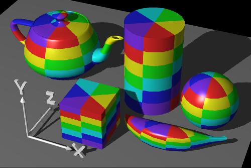
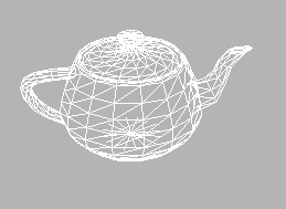
| Polygon | Any closed shape with four or more sides. In 3D, complex objects like teapots are decomposed, or "tessellated", into many primitive polygons to allow regular processing of the data, and hardware acceleration of that processing. |
| Polygon-Based Modelling | Representing 3-D objects as a set or mesh of polygons. |
| Primitives | Smallest units in the 3D database. Usually points, lines, and polygons representing basic geometric shapes, such as balls, cubes, cylinders, and donuts. Some 3D hardware and software schemes also employ curves, known as "splines". |
| QXGA | Quad XGA: a QXGA display has 2048 horizontal pixels and 1536 vertical pixels giving a total display resolution of 3,145,728 individual pixels - 4 times the resolution of an XGA display. |
| Radiosity | Complex methods of drawing 3D scenes, which result in photorealistic images. Essentially, they calculate the path that light rays follow from objects to the viewer, and all the accompanying reflections. Also known as ray tracing. |
| RAMDAC | The RAMDAC converts the data in the frame buffer into the RGB signal required by the monitor. |
| Rasterisation | Rasterisation is the conversion of a polygon 3D scene, stored in a frame buffer, into an image complete with textures, depth cues and lighting. |
| Refresh Rate | Expressed in Hertz (Hz), in interlaced mode this is the number of fields written to the screen every second. In non-interlaced mode it is the number of frames (complete pictures) written to the screen every second. Higher frequencies reduce flicker, because they light the pixels more frequently, reducing the dimming that causes flicker. Also called vertical frequency. |
| Rendering | Fundamentally this relates to the drawing of a real-world object as it actually appears. It often refers to the process of translating high-level database descriptions to bitmap images comprising a matrix of pixels or dots. |
| Resolution | The number of pixels per unit of area. A display with a finer grid contains more pixels and has a higher resolution, capable of reproducing more detail in an image. More of an image can be seen, reducing the need for scrolling or panning. |
| Saturated Colours | Strong, bright colours (particularly reds and oranges) which do not reproduce well on video; they tend to saturate the screen with colour or bleed around the edges, producing a garish, unclear image. |
| Saturation | The colourfulness of an area judged in proportion to its brightness. For example, a fully saturated red would be a pure red. The less saturated, the more pastel the appearance. See also Chroma. |
| Scaling | Process of uniformly changing the size of characters or graphics. |
| Setup | The conversion of a set of instructions concerning the size, shape and position of polygons into a 3D scene ready for rasterisation. |
| Shading | The process of creating pixel colours. Gouraud is a constant increment of colour from one pixel to the next, while Phong is much more complex and higher quality. Flat shading means no smooth blending of colours, each polygon being a single colour. |
| Specular Highlights | A lighting characteristic that determines how light should reflect off an object. Specular highlights are typically white and can move around an object based on camera position. |
| Spline | A 3D bezier curve used in modelling. |
| Spline-Based Modelling | Representing 3-D objects as surfaces made up of mathematically derived curves (splines). |
| Sprite | A small graphic drawn independently of the rest of the screen. |
| SVGA | Super-VGA; when SVGA first came out it was used to describe graphics adapters capable of handling a resolution of 800x600 with support for 256 colours or 1024x768 with 16-colour support. It subsequently came to be used to indicate a capability of 800x600 or greater, regardless of the number of colours available. |
| SXGA | Super XGA: a screen resolution of 1280x1024 pixels, regardless of the number of colours available. |
| Tessellation | The process of dividing an object or surface into geometric primitives (triangles, quadrilaterals, or other polygons) for simplified processing and rendering. |
| Texel | A textured picture element; the basic unit of measurement when dealing with texture-mapped 3D objects. |
| Texture | A (2 dimensional) bitmap pasted onto objects or polygons, to add realism. |
| Texture Filtering | Bilinear or trilinear filtering. Also known as sub-texel positioning. If a pixel is in between texels, the program colours the pixel with an average of the texels’ colours instead of assigning it the exact colour of one single texel. If this is not done, the texture gets very blocky up close as multiple pixels get the exact same texel colouring, while the texture shimmers at a distance because small position changes keep producing large texel changes. |
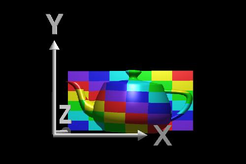
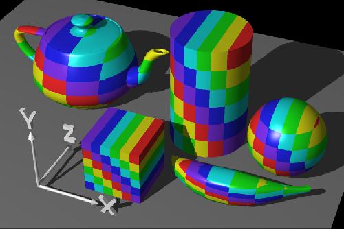
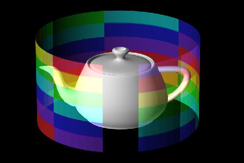
| Texture Mapping | The application of a bitmap onto a 3D shape to give the impression of perspective and different surfaces. Texture maps can vary in size and detail, and can be ‘projected’ on to a shape in various different ways: cylindrically, spherically and so on. |
| Texture Memory | Memory used to store or buffer textures to be mapped on to 3D polygon objects. |
| TIFF | Tagged Image File Format: a popular file format for bitmapped graphics that stores the information defining graphical images in discrete blocks called tags. Each tag describes a particular attribute of the image, such as its width or height, the compression method used (if any), a textual description of the image, or offsets from the start of the file to "strips" containing pixel data. The TIFF format is generic enough to describe virtually any type of bitmap generated on any computer. |
| Time Line | A scale measured in either frames or seconds; it provides an editable record of animation events in time and in sequence. |
| Transparency | The quality of being able to see through a material. The terms transparency and translucency are often used synonymously; however, transparent would technically mean "seeing through clear glass," while translucent would mean "seeing through frosted glass." |
| Trichromatic | The technical name for RGB representation of colour to create all the colours in the spectrum. |
| True Colour | The ability to generate 16,777,216 colours (24-bit colour). |
| Tweening | Also known as in-betweening; calculating the intermediate frames between two keyframes to simulate smooth motion. |
| UXGA | Ultra XGA: a screen resolution of 1600x1200 pixels. |
| Vector Graphics | Images defined by sets of straight lines, defined by the locations of the end points. |
| Vertex | A dimensionless position in three- or four-dimensional space at which two or more lines (for instance, edges) intersect. |
| VESA | Video Electronics Standards Association: an international non-profit organisation established in 1989 to set and support industry-wide interface standards designed for the PC, workstation, and other computing environments. The VESA Local Bus (VL-Bus) standard - introduced in 1992 and widely used before the advent of PCI - was a 32-bit local bus standard compatible with both ISA and EISA cards. |
| VGA | Video Graphics Array: also referred to as Video Graphics Adapter. VGA quickly replaced earlier standards such as CGA (Colour Graphics Adapter) and EGA (Enhanced Graphics Adapter) and made the 640x480 display showing 16 colours the norm. Other manufacturers have since extended the VGA standard to support more pixels and colours. See also SVGA. |
| VGA Feature Connector | A standard 26-pin plug for passing the VGA signal on to some other device, often a video overlay board. This feature connector cannot pass the high-resolution signal from the card and is limited to VGA. |
| Video Mapping | A feature allowing the mapping of an AVI, MPEG movie or animation on to the surface of a 3D object. |
| Video Memory | The graphics card RAM used in the frame buffer, the Z-buffer and, in some 3D graphics cards, texture memory. Common types include DRAM, EDO DRAM, VRAM and WRAM. |
| Video Scaling and Interpolation | When scaled upwards, video clips tend to become pixelated, resulting in block image. Hardware scaling and interpolation routines smooth out these jagged artefacts to create a more realistic picture. Better interpolation routines work on both the X and Y axis to prevent stepping on curved and diagonal elements. |
| Virtual Desktop | When a graphics card is capable of holding in its memory a resolution greater than that being displayed on the screen, the monitor can act as a ‘window’ onto the larger viewing area which may be panned across the "desktop". |
| VM Channel | Vesa Media Channel, VESA's video bus which avoids the main system bus. |
| VRML | Virtual Reality Modelling Language: a database description language applied to create 3D worlds. A standard for Internet-based 3D modelling, but still evolving. |
| VUMA | VESA Unified Memory Architecture: a standard which establishes the electrical and logical interface between a system controller and an external VUMA device enabling them to share physical system memory. |
| Wireframe | All 3D models are constructed from lines and vertices forming a dimensional map of the image. Then texture, shading or motion can be applied. Also referred to as Polygon Mesh. |
| WMF | Windows Meta File: a vector graphics format used mostly for word processing clip art. |
| X Windows | A windowing system developed at MIT, which runs under UNIX and all major operating systems. It uses a client-server protocol and lets users run applications on other computers in the network and view the output on their own screen. |
| XGA | eXtended Graphics Array: also referred to as Extended Graphics Adapter. An IBM graphics standard introduced in 1990 that provides screen pixel resolution of 1024x768 in 256 colours or 640x480 in high (16-bit) colour. It subsequently came to be used to describe cards and monitors capable of resolutions up to 1024x768, regardless of the number of colours available. |
| XYZ Planes | The three dimensions of space; each is designated by an axis. The x- and y-axes are the 2D co-ordinates, at right angles to each other. The z-axis adds the third dimension. Z-buffers accelerate the rendering of 3D scenes by tracking the depth position of objects and working out which are visible and which are hidden behind other objects. |
| YUV | A colour encoding scheme for natural pictures in which luminance and chrominance are separate. The human eye is less sensitive to colour variations than to intensity variations. YUV allows the encoding of luminance (Y) information at full bandwidth and chrominance (UV) information at half bandwidth. |